Frequently Asked Questions (FAQ)
How do I control the way my DataFrame is displayed?
Pandas users rely on a variety of environments for using pandas: scripts, terminal, IPython qtconsole/ notebook, (IDLE, spyder, etc’). Each environment has it’s own capabilities and limitations: HTML support, horizontal scrolling, auto-detection of width/height. To appropriately address all these environments, the display behavior is controlled by several options, which you’re encouraged to tweak to suit your setup.
As of 0.13, these are the relevant options, all under the display namespace, (e.g. display.width, etc.):
- notebook_repr_html: if True, IPython frontends with HTML support will display dataframes as HTML tables when possible.
- large_repr (default ‘truncate’): when a DataFrame exceeds max_columns or max_rows, it can be displayed either as a truncated table or, with this set to ‘info’, as a short summary view.
- max_columns (default 20): max dataframe columns to display.
- max_rows (default 60): max dataframe rows display.
Two additional options only apply to displaying DataFrames in terminals, not to the HTML view:
- expand_repr (default True): when the frame width cannot fit within the screen, the output will be broken into multiple pages.
- width: width of display screen in characters, used to determine the width of lines when expand_repr is active. Setting this to None will trigger auto-detection of terminal width.
IPython users can use the IPython startup file to import pandas and set these options automatically when starting up.
Adding Features to your Pandas Installation
Pandas is a powerful tool and already has a plethora of data manipulation operations implemented, most of them are very fast as well. It’s very possible however that certain functionality that would make your life easier is missing. In that case you have several options:
Open an issue on Github , explain your need and the sort of functionality you would like to see implemented.
Fork the repo, Implement the functionality yourself and open a PR on Github.
Write a method that performs the operation you are interested in and Monkey-patch the pandas class as part of your IPython profile startup or PYTHONSTARTUP file.
For example, here is an example of adding an just_foo_cols() method to the dataframe class:
In [1]: import pandas as pd

In [2]: def just_foo_cols(self):
   ...:     """Get a list of column names containing the string 'foo'
   ...:     """
   ...:     return [x for x in self.columns if 'foo' in x]
   ...:

In [3]: pd.DataFrame.just_foo_cols = just_foo_cols # monkey-patch the DataFrame class

In [4]: df = pd.DataFrame([list(range(4))], columns=["A","foo","foozball","bar"])

In [5]: df.just_foo_cols()
['foo', 'foozball']

In [6]: del pd.DataFrame.just_foo_cols # you can also remove the new method
Monkey-patching is usually frowned upon because it makes your code less portable and can cause subtle bugs in some circumstances. Monkey-patching existing methods is usually a bad idea in that respect. When used with proper care, however, it’s a very useful tool to have.
Migrating from scikits.timeseries to pandas >= 0.8.0
Starting with pandas 0.8.0, users of scikits.timeseries should have all of the features that they need to migrate their code to use pandas. Portions of the scikits.timeseries codebase for implementing calendar logic and timespan frequency conversions (but not resampling, that has all been implemented from scratch from the ground up) have been ported to the pandas codebase.
The scikits.timeseries notions of Date and DateArray are responsible for implementing calendar logic:
In [16]: dt = ts.Date('Q', '1984Q3')

# sic
In [17]: dt
Out[17]: <Q-DEC : 1984Q1>

In [18]: dt.asfreq('D', 'start')
Out[18]: <D : 01-Jan-1984>

In [19]: dt.asfreq('D', 'end')
Out[19]: <D : 31-Mar-1984>

In [20]: dt + 3
Out[20]: <Q-DEC : 1984Q4>
Date and DateArray from scikits.timeseries have been reincarnated in pandas Period and PeriodIndex:
In [7]: pnow('D')  # scikits.timeseries.now()
Period('2014-01-03', 'D')

In [8]: Period(year=2007, month=3, day=15, freq='D')
Period('2007-03-15', 'D')

In [9]: p = Period('1984Q3')

In [10]: p
Period('1984Q3', 'Q-DEC')

In [11]: p.asfreq('D', 'start')
Period('1984-07-01', 'D')

In [12]: p.asfreq('D', 'end')
Period('1984-09-30', 'D')

In [13]: (p + 3).asfreq('T') + 6 * 60 + 30
Period('1985-07-01 06:29', 'T')

In [14]: rng = period_range('1990', '2010', freq='A')

In [15]: rng

<class 'pandas.tseries.period.PeriodIndex'>
freq: A-DEC
[1990, ..., 2010]
length: 21

In [16]: rng.asfreq('B', 'end') - 3

<class 'pandas.tseries.period.PeriodIndex'>
freq: B
[1990-12-26, ..., 2010-12-28]
length: 21
| scikits.timeseries | pandas | Notes |
|---|---|---|
| Date | Period | A span of time, from yearly through to secondly |
| DateArray | PeriodIndex | An array of timespans |
| convert | resample | Frequency conversion in scikits.timeseries |
| convert_to_annual | pivot_annual | currently supports up to daily frequency, see GH736 |
PeriodIndex / DateArray properties and functions
The scikits.timeseries DateArray had a number of information properties. Here are the pandas equivalents:
| scikits.timeseries | pandas | Notes |
|---|---|---|
| get_steps | np.diff(idx.values) | |
| has_missing_dates | not idx.is_full | |
| is_full | idx.is_full | |
| is_valid | idx.is_monotonic and idx.is_unique | |
| is_chronological | is_monotonic | |
| arr.sort_chronologically() | idx.order() |
Frequency conversion
Frequency conversion is implemented using the resample method on TimeSeries and DataFrame objects (multiple time series). resample also works on panels (3D). Here is some code that resamples daily data to montly with scikits.timeseries:
In [17]: import scikits.timeseries as ts

In [18]: data = ts.time_series(np.random.randn(50), start_date='Jan-2000', freq='M')

In [19]: data

timeseries([ 0.4691 -0.2829 -1.5091 -1.1356  1.2121 -0.1732  0.1192 -1.0442 -0.8618
 -2.1046 -0.4949  1.0718  0.7216 -0.7068 -1.0396  0.2719 -0.425   0.567
  0.2762 -1.0874 -0.6737  0.1136 -1.4784  0.525   0.4047  0.577  -1.715
 -1.0393 -0.3706 -1.1579 -1.3443  0.8449  1.0758 -0.109   1.6436 -1.4694
  0.357  -0.6746 -1.7769 -0.9689 -1.2945  0.4137  0.2767 -0.472  -0.014
 -0.3625 -0.0062 -0.9231  0.8957  0.8052],
   dates = [Jan-2014 ... Feb-2018],
   freq  = M)

In [20]: data.convert('A', func=np.mean)

timeseries([-0.3945096205751429 -0.24462765889025218 -0.22163251299635775
 -0.4537726933838235 0.8504806638002349],
   dates = [2014 ... 2018],
   freq  = A-DEC)
Here is the equivalent pandas code:
In [21]: rng = period_range('Jan-2000', periods=50, freq='M')

In [22]: data = Series(np.random.randn(50), index=rng)

In [23]: data

2000-01   -1.206412
2000-02    2.565646
2000-03    1.431256
2000-04    1.340309
2000-05   -1.170299
...
2003-09   -2.179861
2003-10   -1.369849
2003-11   -0.954208
2003-12    1.462696
2004-01   -1.743161
2004-02   -0.826591
Freq: M, Length: 50

In [24]: data.resample('A', how=np.mean)

2000    0.166630
2001   -0.114581
2002   -0.205961
2003   -0.235802
2004   -1.284876
Freq: A-DEC, dtype: float64
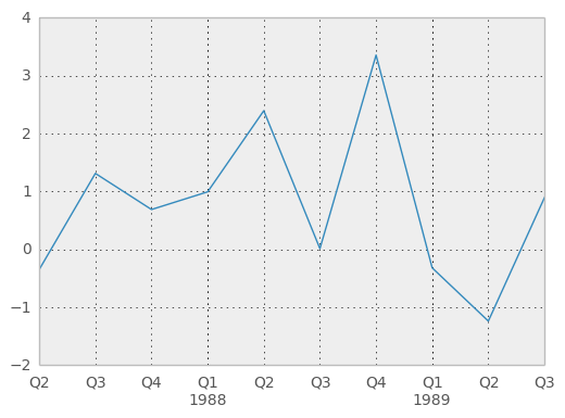
Plotting
Much of the plotting functionality of scikits.timeseries has been ported and adopted to pandas’s data structures. For example:
In [25]: rng = period_range('1987Q2', periods=10, freq='Q-DEC')

In [26]: data = Series(np.random.randn(10), index=rng)

In [27]: plt.figure(); data.plot()
<matplotlib.axes.AxesSubplot at 0x7f5cb90>
Converting to and from period format
Use the to_timestamp and to_period instance methods.
Treatment of missing data
Unlike scikits.timeseries, pandas data structures are not based on NumPy’s MaskedArray object. Missing data is represented as NaN in numerical arrays and either as None or NaN in non-numerical arrays. Implementing a version of pandas’s data structures that use MaskedArray is possible but would require the involvement of a dedicated maintainer. Active pandas developers are not interested in this.
Resampling with timestamps and periods
resample has a kind argument which allows you to resample time series with a DatetimeIndex to PeriodIndex:
In [28]: rng = date_range('1/1/2000', periods=200, freq='D')

In [29]: data = Series(np.random.randn(200), index=rng)

In [30]: data[:10]

2000-01-01   -0.487602
2000-01-02   -0.082240
2000-01-03   -2.182937
2000-01-04    0.380396
2000-01-05    0.084844
2000-01-06    0.432390
2000-01-07    1.519970
2000-01-08   -0.493662
2000-01-09    0.600178
2000-01-10    0.274230
Freq: D, dtype: float64

In [31]: data.index

<class 'pandas.tseries.index.DatetimeIndex'>
[2000-01-01 00:00:00, ..., 2000-07-18 00:00:00]
Length: 200, Freq: D, Timezone: None

In [32]: data.resample('M', kind='period')

2000-01    0.163775
2000-02    0.026549
2000-03   -0.089563
2000-04   -0.079405
2000-05    0.160348
2000-06    0.101725
2000-07   -0.708770
Freq: M, dtype: float64
Similarly, resampling from periods to timestamps is possible with an optional interval ('start' or 'end') convention:
In [33]: rng = period_range('Jan-2000', periods=50, freq='M')

In [34]: data = Series(np.random.randn(50), index=rng)

In [35]: resampled = data.resample('A', kind='timestamp', convention='end')

In [36]: resampled.index

<class 'pandas.tseries.index.DatetimeIndex'>
[2000-12-31 00:00:00, ..., 2004-12-31 00:00:00]
Length: 5, Freq: A-DEC, Timezone: None
Byte-Ordering Issues
Occasionally you may have to deal with data that were created on a machine with a different byte order than the one on which you are running Python. To deal with this issue you should convert the underlying NumPy array to the native system byte order before passing it to Series/DataFrame/Panel constructors using something similar to the following:
In [37]: x = np.array(list(range(10)), '>i4') # big endian

In [38]: newx = x.byteswap().newbyteorder() # force native byteorder

In [39]: s = Series(newx)
See the NumPy documentation on byte order for more details.
Visualizing Data in Qt applications
There is experimental support for visualizing DataFrames in PyQt4 and PySide applications. At the moment you can display and edit the values of the cells in the DataFrame. Qt will take care of displaying just the portion of the DataFrame that is currently visible and the edits will be immediately saved to the underlying DataFrame
To demonstrate this we will create a simple PySide application that will switch between two editable DataFrames. For this will use the DataFrameModel class that handles the access to the DataFrame, and the DataFrameWidget, which is just a thin layer around the QTableView.
import numpy as np
import pandas as pd
from pandas.sandbox.qtpandas import DataFrameModel, DataFrameWidget
from PySide import QtGui, QtCore

# Or if you use PyQt4:
# from PyQt4 import QtGui, QtCore

class MainWidget(QtGui.QWidget):
    def __init__(self, parent=None):
        super(MainWidget, self).__init__(parent)

        # Create two DataFrames
        self.df1 = pd.DataFrame(np.arange(9).reshape(3, 3),
                                columns=['foo', 'bar', 'baz'])
        self.df2 = pd.DataFrame({
                'int': [1, 2, 3],
                'float': [1.5, 2.5, 3.5],
                'string': ['a', 'b', 'c'],
                'nan': [np.nan, np.nan, np.nan]
            }, index=['AAA', 'BBB', 'CCC'],
            columns=['int', 'float', 'string', 'nan'])

        # Create the widget and set the first DataFrame
        self.widget = DataFrameWidget(self.df1)

        # Create the buttons for changing DataFrames
        self.button_first = QtGui.QPushButton('First')
        self.button_first.clicked.connect(self.on_first_click)
        self.button_second = QtGui.QPushButton('Second')
        self.button_second.clicked.connect(self.on_second_click)

        # Set the layout
        vbox = QtGui.QVBoxLayout()
        vbox.addWidget(self.widget)
        hbox = QtGui.QHBoxLayout()
        hbox.addWidget(self.button_first)
        hbox.addWidget(self.button_second)
        vbox.addLayout(hbox)
        self.setLayout(vbox)

    def on_first_click(self):
        '''Sets the first DataFrame'''
        self.widget.setDataFrame(self.df1)

    def on_second_click(self):
        '''Sets the second DataFrame'''
        self.widget.setDataFrame(self.df2)

if __name__ == '__main__':
    import sys

    # Initialize the application
    app = QtGui.QApplication(sys.argv)
    mw = MainWidget()
    mw.show()
    app.exec_()