Computational tools
Statistical functions
Covariance
The Series object has a method cov to compute covariance between series (excluding NA/null values).
In [157]: s1 = Series(randn(1000))

In [158]: s2 = Series(randn(1000))

In [159]: s1.cov(s2)
Out[159]: 0.019465636696791695
Analogously, DataFrame has a method cov to compute pairwise covariances among the series in the DataFrame, also excluding NA/null values.
In [160]: frame = DataFrame(randn(1000, 5), columns=['a', 'b', 'c', 'd', 'e'])

In [161]: frame.cov()
Out[161]:
          a         b         c         d         e
a  0.953751 -0.029550 -0.006415  0.001020 -0.004134
b -0.029550  0.997223 -0.044276  0.005967  0.044884
c -0.006415 -0.044276  1.050236  0.077775  0.010642
d  0.001020  0.005967  0.077775  0.998485 -0.007345
e -0.004134  0.044884  0.010642 -0.007345  1.025446
Correlation
Several methods for computing correlations are provided. Several kinds of correlation methods are provided:
| Method name | Description |
|---|---|
| pearson (default) | Standard correlation coefficient |
| kendall | Kendall Tau correlation coefficient |
| spearman | Spearman rank correlation coefficient |
All of these are currently computed using pairwise complete observations.
In [162]: frame = DataFrame(randn(1000, 5), columns=['a', 'b', 'c', 'd', 'e'])

In [163]: frame.ix[::2] = np.nan

# Series with Series
In [164]: frame['a'].corr(frame['b'])
Out[164]: 0.013306883832198543

In [165]: frame['a'].corr(frame['b'], method='spearman')
Out[165]: 0.022530330121320486

# Pairwise correlation of DataFrame columns
In [166]: frame.corr()
Out[166]:
          a         b         c         d         e
a  1.000000  0.013307 -0.037801 -0.021905  0.001165
b  0.013307  1.000000 -0.017259  0.079246 -0.043606
c -0.037801 -0.017259  1.000000  0.061657  0.078945
d -0.021905  0.079246  0.061657  1.000000 -0.036978
e  0.001165 -0.043606  0.078945 -0.036978  1.000000
Note that non-numeric columns will be automatically excluded from the correlation calculation.
A related method corrwith is implemented on DataFrame to compute the correlation between like-labeled Series contained in different DataFrame objects.
In [167]: index = ['a', 'b', 'c', 'd', 'e']

In [168]: columns = ['one', 'two', 'three', 'four']

In [169]: df1 = DataFrame(randn(5, 4), index=index, columns=columns)

In [170]: df2 = DataFrame(randn(4, 4), index=index[:4], columns=columns)

In [171]: df1.corrwith(df2)
Out[171]:
one      0.344149
two      0.837438
three    0.458904
four     0.712401

In [172]: df2.corrwith(df1, axis=1)
Out[172]:
a    0.404019
b    0.772204
c    0.420390
d   -0.142959
e         NaN
Data ranking
The rank method produces a data ranking with ties being assigned the mean of the ranks for the group:
In [173]: s = Series(np.random.randn(5), index=list('abcde'))

In [174]: s['d'] = s['b'] # so there's a tie

In [175]: s.rank()
Out[175]:
a    2.0
b    3.5
c    1.0
d    3.5
e    5.0
rank is also a DataFrame method and can rank either the rows (axis=0) or the columns (axis=1). NaN values are excluded from the ranking.
In [176]: df = DataFrame(np.random.randn(10, 6))

In [177]: df[4] = df[2][:5] # some ties

In [178]: df
Out[178]:
          0         1         2         3         4         5
0  0.106333  0.712162 -0.351275  1.176287 -0.351275  1.741787
1 -1.301869  0.612432 -0.577677  0.124709 -0.577677 -1.068084
2 -0.899627  0.822023  1.506319  0.998896  1.506319  0.259080
3 -0.522705 -1.473680 -1.726800  1.555343 -1.726800 -1.411978
4  0.733147  0.415881 -0.026973  0.999488 -0.026973  0.082219
5  0.995001 -1.399355  0.082244 -1.521795       NaN  0.416180
6 -0.779714 -0.226893  0.956567 -0.443664       NaN -0.610675
7 -0.635495 -0.621647  0.406259 -0.279002       NaN -1.153000
8  0.085011 -0.459422 -1.660917 -1.913019       NaN  0.833479
9 -0.557052  0.775425  0.003794  0.555351       NaN -1.169977

In [179]: df.rank(1)
Out[179]:
   0  1    2  3    4  5
0  3  4  1.5  5  1.5  6
1  1  6  3.5  5  3.5  2
2  1  3  5.5  4  5.5  2
3  5  3  1.5  6  1.5  4
4  5  4  1.5  6  1.5  3
5  5  2  3.0  1  NaN  4
6  1  4  5.0  3  NaN  2
7  2  3  5.0  4  NaN  1
8  4  3  2.0  1  NaN  5
9  2  5  3.0  4  NaN  1
Note
These methods are significantly faster (around 10-20x) than scipy.stats.rankdata.
Moving (rolling) statistics / moments
For working with time series data, a number of functions are provided for computing common moving or rolling statistics. Among these are count, sum, mean, median, correlation, variance, covariance, standard deviation, skewness, and kurtosis. All of these methods are in the pandas namespace, but otherwise they can be found in pandas.stats.moments.
| Function | Description |
|---|---|
| rolling_count | Number of non-null observations |
| rolling_sum | Sum of values |
| rolling_mean | Mean of values |
| rolling_median | Arithmetic median of values |
| rolling_min | Minimum |
| rolling_max | Maximum |
| rolling_std | Unbiased standard deviation |
| rolling_var | Unbiased variance |
| rolling_skew | Unbiased skewness (3rd moment) |
| rolling_kurt | Unbiased kurtosis (4th moment) |
| rolling_quantile | Sample quantile (value at %) |
| rolling_apply | Generic apply |
| rolling_cov | Unbiased covariance (binary) |
| rolling_corr | Correlation (binary) |
| rolling_corr_pairwise | Pairwise correlation of DataFrame columns |
Generally these methods all have the same interface. The binary operators (e.g. rolling_corr) take two Series or DataFrames. Otherwise, they all accept the following arguments:
- window: size of moving window
- min_periods: threshold of non-null data points to require (otherwise result is NA)
- time_rule: optionally specify a time rule to pre-conform the data to
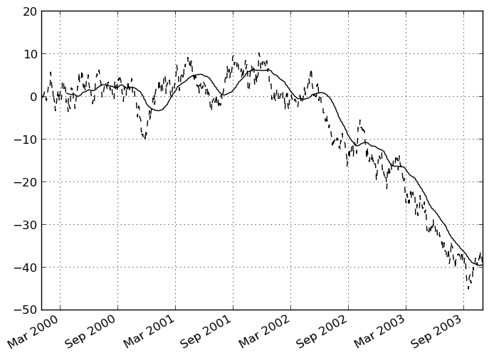
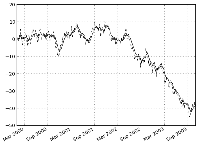
These functions can be applied to ndarrays or Series objects:
In [180]: ts = Series(randn(1000), index=DateRange('1/1/2000', periods=1000))

In [181]: ts = ts.cumsum()

In [182]: ts.plot(style='k--')
Out[182]: <matplotlib.axes.AxesSubplot at 0x10a7bad10>

In [183]: rolling_mean(ts, 60).plot(style='k')
Out[183]: <matplotlib.axes.AxesSubplot at 0x10a7bad10>
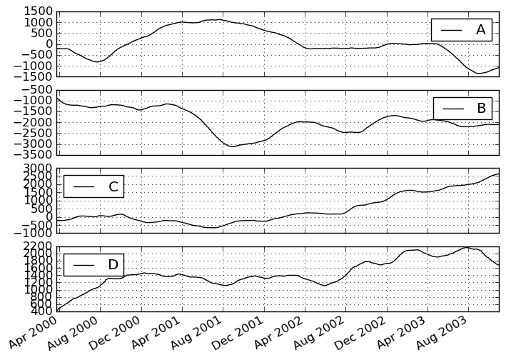
They can also be applied to DataFrame objects. This is really just syntactic sugar for applying the moving window operator to all of the DataFrame’s columns:
In [184]: df = DataFrame(randn(1000, 4), index=ts.index,
   .....:                columns=['A', 'B', 'C', 'D'])

In [185]: df = df.cumsum()

In [186]: rolling_sum(df, 60).plot(subplots=True)
Out[186]:
array([Axes(0.125,0.747826;0.775x0.152174),
       Axes(0.125,0.565217;0.775x0.152174),
       Axes(0.125,0.382609;0.775x0.152174), Axes(0.125,0.2;0.775x0.152174)], dtype=object)
Binary rolling moments
rolling_cov and rolling_corr can compute moving window statistics about two Series or any combination of DataFrame/Series or DataFrame/DataFrame. Here is the behavior in each case:
- two Series: compute the statistic for the pairing
- DataFrame/Series: compute the statistics for each column of the DataFrame with the passed Series, thus returning a DataFrame
- DataFrame/DataFrame: compute statistic for matching column names, returning a DataFrame
For example:
In [187]: df2 = df[:20]

In [188]: rolling_corr(df2, df2['B'], window=5)
Out[188]:
                   A   B         C         D
2000-01-03       NaN NaN       NaN       NaN
2000-01-04       NaN NaN       NaN       NaN
2000-01-05       NaN NaN       NaN       NaN
2000-01-06       NaN NaN       NaN       NaN
2000-01-07  0.806980   1 -0.911973 -0.747745
2000-01-10  0.689915   1 -0.609054 -0.680394
2000-01-11  0.211679   1 -0.383565 -0.164879
2000-01-12  0.286270   1  0.104075  0.345844
2000-01-13 -0.565249   1  0.039148  0.333921
2000-01-14  0.295310   1  0.501143 -0.524100
2000-01-17  0.041252   1  0.868636 -0.577590
2000-01-18  0.205705   1  0.917778 -0.819271
2000-01-19  0.326449   1  0.933352 -0.882750
2000-01-20  0.120893   1  0.409255 -0.795062
2000-01-21  0.680531   1 -0.192045 -0.349044
2000-01-24  0.643667   1 -0.588676  0.473287
2000-01-25  0.703188   1 -0.746130  0.714265
2000-01-26  0.065322   1 -0.209789  0.635360
2000-01-27 -0.429914   1 -0.100807  0.266005
2000-01-28 -0.387498   1  0.512321  0.592033
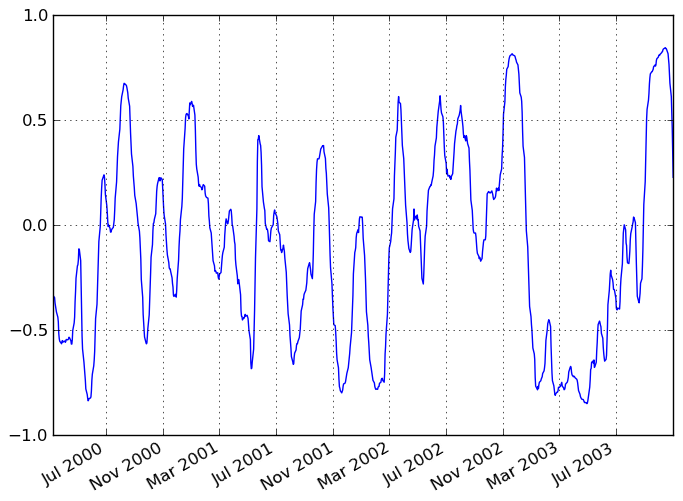
Computing rolling pairwise correlations
In financial data analysis and other fields it’s common to compute correlation matrices for a collection of time series. More difficult is to compute a moving-window correlation matrix. This can be done using the rolling_corr_pairwise function, which yields a Panel whose items are the dates in question:
In [189]: correls = rolling_corr_pairwise(df, 50)

In [190]: correls[df.index[-50]]
Out[190]:
          A         B         C         D
A  1.000000 -0.177708 -0.253742  0.303872
B -0.177708  1.000000 -0.085484  0.008572
C -0.253742 -0.085484  1.000000 -0.769233
D  0.303872  0.008572 -0.769233  1.000000
You can efficiently retrieve the time series of correlations between two columns using ix indexing:
In [191]: correls.ix[:, 'A', 'C'].plot()
Out[191]: <matplotlib.axes.AxesSubplot at 0x10f85a910>
Exponentially weighted moment functions
A related set of functions are exponentially weighted versions of many of the
above statistics. A number of EW (exponentially weighted) functions are
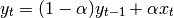
provided using the blending method. For example, where  is the
result and
is the
result and  the input, we compute an exponentially weighted moving
average as
the input, we compute an exponentially weighted moving
average as
One must have  , but rather than pass
  directly, it’s easier to think about either the span or center of mass
(com) of an EW moment:
directly, it’s easier to think about either the span or center of mass
(com) of an EW moment:
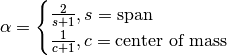
You can pass one or the other to these functions but not both. Span corresponds to what is commonly called a “20-day EW moving average” for example. Center of mass has a more physical interpretation. For example, span = 20 corresponds to com = 9.5. Here is the list of functions available:
| Function | Description |
|---|---|
| ewma | EW moving average |
| ewvar | EW moving variance |
| ewstd | EW moving standard deviation |
| ewmcorr | EW moving correlation |
| ewmcov | EW moving covariance |
Here are an example for a univariate time series:
In [192]: plt.close('all')

In [193]: ts.plot(style='k--')
Out[193]: <matplotlib.axes.AxesSubplot at 0x10f86c610>

In [194]: ewma(ts, span=20).plot(style='k')
Out[194]: <matplotlib.axes.AxesSubplot at 0x10f86c610>
Note
The EW functions perform a standard adjustment to the initial observations whereby if there are fewer observations than called for in the span, those observations are reweighted accordingly.
Linear and panel regression
Note
We plan to move this functionality to statsmodels for the next release. Some of the result attributes may change names in order to foster naming consistency with the rest of statsmodels. We will provide every effort to provide compatibility with older versions of pandas, however.
We have implemented a very fast set of moving-window linear regression classes in pandas. Two different types of regressions are supported:
- Standard ordinary least squares (OLS) multiple regression
- Multiple regression (OLS-based) on panel data including with fixed-effects (also known as entity or individual effects) or time-effects.
Both kinds of linear models are accessed through the ols function in the pandas namespace. They all take the following arguments to specify either a static (full sample) or dynamic (moving window) regression:
- window_type: 'full sample' (default), 'expanding', or rolling
- window: size of the moving window in the window_type='rolling' case. If window is specified, window_type will be automatically set to 'rolling'
- min_periods: minimum number of time periods to require to compute the regression coefficients
Generally speaking, the ols works by being given a y (response) object and an x (predictors) object. These can take many forms:
- y: a Series, ndarray, or DataFrame (panel model)
- x: Series, DataFrame, dict of Series, dict of DataFrame or Panel
Based on the types of y and x, the model will be inferred to either a panel model or a regular linear model. If the y variable is a DataFrame, the result will be a panel model. In this case, the x variable must either be a Panel, or a dict of DataFrame (which will be coerced into a Panel).
Standard OLS regression
Let’s pull in some sample data:
In [195]: from pandas.io.data import DataReader

In [196]: symbols = ['MSFT', 'GOOG', 'AAPL']

In [197]: data = dict((sym, DataReader(sym, "yahoo"))
   .....:             for sym in symbols)

In [198]: panel = Panel(data).swapaxes('items', 'minor')

In [199]: close_px = panel['Close']

# convert closing prices to returns
In [200]: rets = close_px / close_px.shift(1) - 1

In [201]: rets.info()
<class 'pandas.core.frame.DataFrame'>
Index: 250 entries, 2011-11-09 00:00:00 to 2012-11-07 00:00:00
Data columns:
AAPL    249  non-null values
GOOG    249  non-null values
MSFT    249  non-null values
dtypes: float64(3)
Let’s do a static regression of AAPL returns on GOOG returns:
In [202]: model = ols(y=rets['AAPL'], x=rets.ix[:, ['GOOG']])

In [203]: model
Out[203]:
-------------------------Summary of Regression Analysis-------------------------
Formula: Y ~ <GOOG> + <intercept>
Number of Observations:         249
Number of Degrees of Freedom:   2
R-squared:         0.1691
Adj R-squared:     0.1658
Rmse:              0.0157
F-stat (1, 247):    50.2798, p-value:     0.0000
Degrees of Freedom: model 1, resid 247
-----------------------Summary of Estimated Coefficients------------------------
      Variable       Coef    Std Err     t-stat    p-value    CI 2.5%   CI 97.5%
--------------------------------------------------------------------------------
          GOOG     0.4791     0.0676       7.09     0.0000     0.3466     0.6115
     intercept     0.0013     0.0010       1.28     0.2012    -0.0007     0.0032
---------------------------------End of Summary---------------------------------

In [204]: model.beta
Out[204]:
GOOG         0.479054
intercept    0.001278
If we had passed a Series instead of a DataFrame with the single GOOG column, the model would have assigned the generic name x to the sole right-hand side variable.
We can do a moving window regression to see how the relationship changes over time:
In [205]: model = ols(y=rets['AAPL'], x=rets.ix[:, ['GOOG']],
   .....:             window=250)

# just plot the coefficient for GOOG
In [206]: model.beta['GOOG'].plot()
Out[206]: <matplotlib.axes.AxesSubplot at 0x111df0e50>
It looks like there are some outliers rolling in and out of the window in the above regression, influencing the results. We could perform a simple winsorization at the 3 STD level to trim the impact of outliers:
In [207]: winz = rets.copy()

In [208]: std_1year = rolling_std(rets, 250, min_periods=20)

# cap at 3 * 1 year standard deviation
In [209]: cap_level = 3 * np.sign(winz) * std_1year

In [210]: winz[np.abs(winz) > 3 * std_1year] = cap_level

In [211]: winz_model = ols(y=winz['AAPL'], x=winz.ix[:, ['GOOG']],
   .....:             window=250)

In [212]: model.beta['GOOG'].plot(label="With outliers")
Out[212]: <matplotlib.axes.AxesSubplot at 0x111e09210>

In [213]: winz_model.beta['GOOG'].plot(label="Winsorized"); plt.legend(loc='best')
Out[213]: <matplotlib.legend.Legend at 0x11158c0d0>
So in this simple example we see the impact of winsorization is actually quite significant. Note the correlation after winsorization remains high:
In [214]: winz.corrwith(rets)
Out[214]:
AAPL    0.991873
GOOG    0.984418
MSFT    0.998519
Multiple regressions can be run by passing a DataFrame with multiple columns for the predictors x:
In [215]: ols(y=winz['AAPL'], x=winz.drop(['AAPL'], axis=1))
Out[215]:
-------------------------Summary of Regression Analysis-------------------------
Formula: Y ~ <GOOG> + <MSFT> + <intercept>
Number of Observations:         249
Number of Degrees of Freedom:   3
R-squared:         0.2347
Adj R-squared:     0.2285
Rmse:              0.0144
F-stat (2, 246):    37.7281, p-value:     0.0000
Degrees of Freedom: model 2, resid 246
-----------------------Summary of Estimated Coefficients------------------------
      Variable       Coef    Std Err     t-stat    p-value    CI 2.5%   CI 97.5%
--------------------------------------------------------------------------------
          GOOG     0.4502     0.0712       6.32     0.0000     0.3107     0.5897
          MSFT     0.2654     0.0748       3.55     0.0005     0.1188     0.4120
     intercept     0.0009     0.0009       0.94     0.3482    -0.0009     0.0027
---------------------------------End of Summary---------------------------------
Panel regression
We’ve implemented moving window panel regression on potentially unbalanced panel data (see this article if this means nothing to you). Suppose we wanted to model the relationship between the magnitude of the daily return and trading volume among a group of stocks, and we want to pool all the data together to run one big regression. This is actually quite easy:
# make the units somewhat comparable
In [216]: volume = panel['Volume'] / 1e8

In [217]: model = ols(y=volume, x={'return' : np.abs(rets)})

In [218]: model
Out[218]:
-------------------------Summary of Regression Analysis-------------------------
Formula: Y ~ <return> + <intercept>
Number of Observations:         747
Number of Degrees of Freedom:   2
R-squared:         0.0244
Adj R-squared:     0.0231
Rmse:              0.2105
F-stat (1, 745):    18.6418, p-value:     0.0000
Degrees of Freedom: model 1, resid 745
-----------------------Summary of Estimated Coefficients------------------------
      Variable       Coef    Std Err     t-stat    p-value    CI 2.5%   CI 97.5%
--------------------------------------------------------------------------------
        return     3.1731     0.7349       4.32     0.0000     1.7327     4.6136
     intercept     0.1888     0.0111      16.95     0.0000     0.1670     0.2107
---------------------------------End of Summary---------------------------------
In a panel model, we can insert dummy (0-1) variables for the “entities” involved (here, each of the stocks) to account the a entity-specific effect (intercept):
In [219]: fe_model = ols(y=volume, x={'return' : np.abs(rets)},
   .....:                entity_effects=True)

In [220]: fe_model
Out[220]:
-------------------------Summary of Regression Analysis-------------------------
Formula: Y ~ <return> + <FE_GOOG> + <FE_MSFT> + <intercept>
Number of Observations:         747
Number of Degrees of Freedom:   4
R-squared:         0.7843
Adj R-squared:     0.7834
Rmse:              0.0991
F-stat (3, 743):   900.6175, p-value:     0.0000
Degrees of Freedom: model 3, resid 743
-----------------------Summary of Estimated Coefficients------------------------
      Variable       Coef    Std Err     t-stat    p-value    CI 2.5%   CI 97.5%
--------------------------------------------------------------------------------
        return     4.0218     0.3483      11.55     0.0000     3.3392     4.7044
       FE_GOOG    -0.1396     0.0089     -15.66     0.0000    -0.1571    -0.1221
       FE_MSFT     0.3052     0.0089      34.16     0.0000     0.2877     0.3227
     intercept     0.1244     0.0077      16.24     0.0000     0.1093     0.1394
---------------------------------End of Summary---------------------------------
Because we ran the regression with an intercept, one of the dummy variables must be dropped or the design matrix will not be full rank. If we do not use an intercept, all of the dummy variables will be included:
In [221]: fe_model = ols(y=volume, x={'return' : np.abs(rets)},
   .....:                entity_effects=True, intercept=False)

In [222]: fe_model
Out[222]:
-------------------------Summary of Regression Analysis-------------------------
Formula: Y ~ <return> + <FE_AAPL> + <FE_GOOG> + <FE_MSFT>
Number of Observations:         747
Number of Degrees of Freedom:   4
R-squared:         0.7843
Adj R-squared:     0.7834
Rmse:              0.0991
F-stat (4, 743):   900.6175, p-value:     0.0000
Degrees of Freedom: model 3, resid 743
-----------------------Summary of Estimated Coefficients------------------------
      Variable       Coef    Std Err     t-stat    p-value    CI 2.5%   CI 97.5%
--------------------------------------------------------------------------------
        return     4.0218     0.3483      11.55     0.0000     3.3392     4.7044
       FE_AAPL     0.1244     0.0077      16.24     0.0000     0.1093     0.1394
       FE_GOOG    -0.0153     0.0073      -2.10     0.0358    -0.0295    -0.0010
       FE_MSFT     0.4295     0.0071      60.08     0.0000     0.4155     0.4436
---------------------------------End of Summary---------------------------------
We can also include time effects, which demeans the data cross-sectionally at each point in time (equivalent to including dummy variables for each date). More mathematical care must be taken to properly compute the standard errors in this case:
In [223]: te_model = ols(y=volume, x={'return' : np.abs(rets)},
   .....:                time_effects=True, entity_effects=True)

In [224]: te_model
Out[224]:
-------------------------Summary of Regression Analysis-------------------------
Formula: Y ~ <return> + <FE_GOOG> + <FE_MSFT>
Number of Observations:         747
Number of Degrees of Freedom:   252
R-squared:         0.8445
Adj R-squared:     0.7656
Rmse:              0.0979
F-stat (3, 495):    10.7076, p-value:     0.0000
Degrees of Freedom: model 251, resid 495
-----------------------Summary of Estimated Coefficients------------------------
      Variable       Coef    Std Err     t-stat    p-value    CI 2.5%   CI 97.5%
--------------------------------------------------------------------------------
        return     3.4851     0.4777       7.30     0.0000     2.5488     4.4214
       FE_GOOG    -0.1408     0.0088     -15.94     0.0000    -0.1581    -0.1235
       FE_MSFT     0.3037     0.0089      34.24     0.0000     0.2863     0.3211
---------------------------------End of Summary---------------------------------
Here the intercept (the mean term) is dropped by default because it will be 0 according to the model assumptions, having subtracted off the group means.
Result fields and tests
We’ll leave it to the user to explore the docstrings and source, especially as we’ll be moving this code into statsmodels in the near future.