Computational tools¶

Statistical functions¶

Percent Change¶

Both Series and DataFrame has a method pct_change to compute the percent change over a given number of periods (using fill_method to fill NA/null values).

In [191]: ser = Series(randn(8))

In [192]: ser.pct_change()
Out[192]: 
       NaN
 -1.602976
  4.334938
 -0.247456
 -2.067345
 -1.142903
 -1.688214
 -9.759729

In [193]: df = DataFrame(randn(10, 4))

In [194]: df.pct_change(periods=3)
Out[194]: 
          0         1         2         3
     NaN       NaN       NaN       NaN
     NaN       NaN       NaN       NaN
     NaN       NaN       NaN       NaN
-0.218320 -1.054001  1.987147 -0.510183
-0.439121 -1.816454  0.649715 -4.822809
-0.127833 -3.042065 -5.866604 -1.776977
-2.596833 -1.959538 -2.111697 -3.798900
-0.117826 -2.169058  0.036094 -0.067696
2.492606 -1.357320 -1.205802 -1.558697
-1.012977  2.324558 -1.003744 -0.371806

Covariance¶

The Series object has a method cov to compute covariance between series (excluding NA/null values).

In [195]: s1 = Series(randn(1000))

In [196]: s2 = Series(randn(1000))

In [197]: s1.cov(s2)
Out[197]: 0.00068010881743110524

Analogously, DataFrame has a method cov to compute pairwise covariances among the series in the DataFrame, also excluding NA/null values.

In [198]: frame = DataFrame(randn(1000, 5), columns=['a', 'b', 'c', 'd', 'e'])

In [199]: frame.cov()
Out[199]: 
          a         b         c         d         e
a  1.000882 -0.003177 -0.002698 -0.006889  0.031912
b -0.003177  1.024721  0.000191  0.009212  0.000857
c -0.002698  0.000191  0.950735 -0.031743 -0.005087
d -0.006889  0.009212 -0.031743  1.002983 -0.047952
e  0.031912  0.000857 -0.005087 -0.047952  1.042487

Correlation¶

Several methods for computing correlations are provided. Several kinds of correlation methods are provided:

Method name	Description
`pearson (default)`	Standard correlation coefficient
`kendall`	Kendall Tau correlation coefficient
`spearman`	Spearman rank correlation coefficient

All of these are currently computed using pairwise complete observations.

In [200]: frame = DataFrame(randn(1000, 5), columns=['a', 'b', 'c', 'd', 'e'])

In [201]: frame.ix[::2] = np.nan

# Series with Series
In [202]: frame['a'].corr(frame['b'])
Out[202]: 0.010052135416653471

In [203]: frame['a'].corr(frame['b'], method='spearman')
Out[203]: -0.0097383749534998149

# Pairwise correlation of DataFrame columns
In [204]: frame.corr()
Out[204]: 
          a         b         c         d         e
a  1.000000  0.010052 -0.047750 -0.031461 -0.025285
b  0.010052  1.000000 -0.014172 -0.020590 -0.001930
c -0.047750 -0.014172  1.000000  0.006373 -0.049479
d -0.031461 -0.020590  0.006373  1.000000 -0.012379
e -0.025285 -0.001930 -0.049479 -0.012379  1.000000

Note that non-numeric columns will be automatically excluded from the correlation calculation.

A related method corrwith is implemented on DataFrame to compute the correlation between like-labeled Series contained in different DataFrame objects.

In [205]: index = ['a', 'b', 'c', 'd', 'e']

In [206]: columns = ['one', 'two', 'three', 'four']

In [207]: df1 = DataFrame(randn(5, 4), index=index, columns=columns)

In [208]: df2 = DataFrame(randn(4, 4), index=index[:4], columns=columns)

In [209]: df1.corrwith(df2)
Out[209]: 
one      0.803464
two      0.142469
three   -0.498774
four     0.806420

In [210]: df2.corrwith(df1, axis=1)
Out[210]: 
a    0.011572
b    0.388066
c   -0.335819
d    0.232412
e         NaN

Data ranking¶

The rank method produces a data ranking with ties being assigned the mean of the ranks (by default) for the group:

In [211]: s = Series(np.random.randn(5), index=list('abcde'))

In [212]: s['d'] = s['b'] # so there's a tie

In [213]: s.rank()
Out[213]: 
a    2.0
b    4.5
c    3.0
d    4.5
e    1.0

rank is also a DataFrame method and can rank either the rows (axis=0) or the columns (axis=1). NaN values are excluded from the ranking.

In [214]: df = DataFrame(np.random.randn(10, 6))

In [215]: df[4] = df[2][:5] # some ties

In [216]: df
Out[216]: 
          0         1         2         3         4         5
0.085011 -0.459422 -1.660917 -1.913019 -1.660917  0.833479
-0.557052  0.775425  0.003794  0.555351  0.003794 -1.169977
0.815695 -0.295737 -0.534290  0.068917 -0.534290 -0.513855
1.465947  0.021757  0.523224 -0.439297  0.523224 -0.959568
-0.678378  0.091855  1.337956  0.792551  1.337956  0.711776
-0.190285  0.187520 -0.355562  1.730964       NaN -1.362312
-0.776678 -2.082637 -0.165877  0.357163       NaN  0.631662
-1.295037  0.367656 -1.886797 -0.531790       NaN  1.270408
1.106052  0.848312 -0.613544  1.338296       NaN -1.150652
0.309979  1.088439  0.920366 -0.750322       NaN  1.563956

In [217]: df.rank(1)
Out[217]: 
1    2  3    4  5
5  4  2.5  1  2.5  6
2  6  3.5  5  3.5  1
6  4  1.5  5  1.5  3
6  3  4.5  2  4.5  1
1  2  5.5  4  5.5  3
3  4  2.0  5  NaN  1
2  1  3.0  4  NaN  5
2  4  1.0  3  NaN  5
4  3  2.0  5  NaN  1
2  4  3.0  1  NaN  5

rank optionally takes a parameter ascending which by default is true; when false, data is reverse-ranked, with larger values assigned a smaller rank.

rank supports different tie-breaking methods, specified with the method parameter:

average : average rank of tied group

min : lowest rank in the group

max : highest rank in the group

first : ranks assigned in the order they appear in the array

Note

These methods are significantly faster (around 10-20x) than scipy.stats.rankdata.

Moving (rolling) statistics / moments¶

For working with time series data, a number of functions are provided for computing common moving or rolling statistics. Among these are count, sum, mean, median, correlation, variance, covariance, standard deviation, skewness, and kurtosis. All of these methods are in the pandas namespace, but otherwise they can be found in pandas.stats.moments.

Function	Description
`rolling_count`	Number of non-null observations
`rolling_sum`	Sum of values
`rolling_mean`	Mean of values
`rolling_median`	Arithmetic median of values
`rolling_min`	Minimum
`rolling_max`	Maximum
`rolling_std`	Unbiased standard deviation
`rolling_var`	Unbiased variance
`rolling_skew`	Unbiased skewness (3rd moment)
`rolling_kurt`	Unbiased kurtosis (4th moment)
`rolling_quantile`	Sample quantile (value at %)
`rolling_apply`	Generic apply
`rolling_cov`	Unbiased covariance (binary)
`rolling_corr`	Correlation (binary)
`rolling_corr_pairwise`	Pairwise correlation of DataFrame columns

Generally these methods all have the same interface. The binary operators (e.g. rolling_corr) take two Series or DataFrames. Otherwise, they all accept the following arguments:

window: size of moving window

min_periods: threshold of non-null data points to require (otherwise result is NA)

freq: optionally specify a frequency string or DateOffset to pre-conform the data to. Note that prior to pandas v0.8.0, a keyword argument time_rule was used instead of freq that referred to the legacy time rule constants

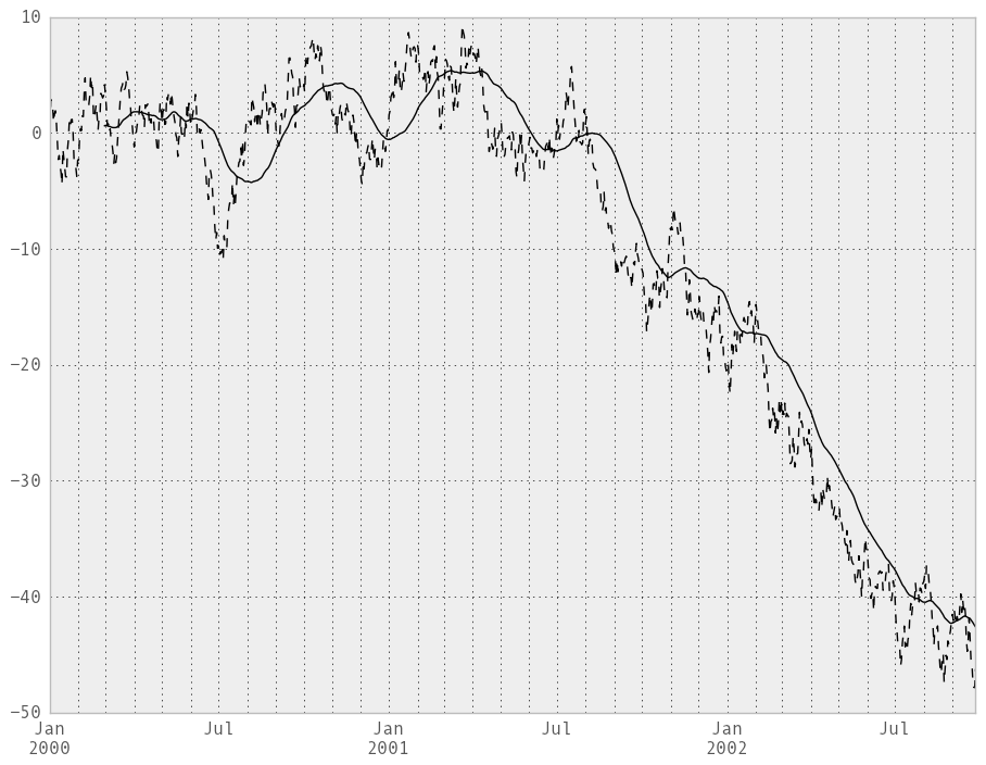
These functions can be applied to ndarrays or Series objects:

In [218]: ts = Series(randn(1000), index=date_range('1/1/2000', periods=1000))

In [219]: ts = ts.cumsum()

In [220]: ts.plot(style='k--')
Out[220]: <matplotlib.axes.AxesSubplot at 0x10a772210>

In [221]: rolling_mean(ts, 60).plot(style='k')
Out[221]: <matplotlib.axes.AxesSubplot at 0x10a772210>

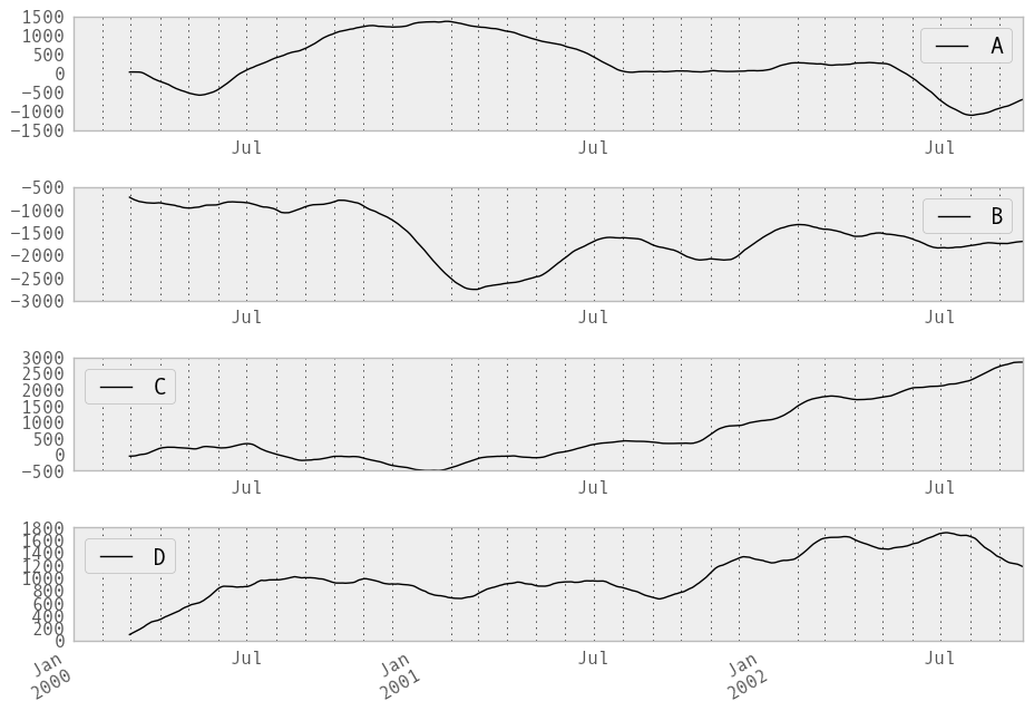
They can also be applied to DataFrame objects. This is really just syntactic sugar for applying the moving window operator to all of the DataFrame’s columns:

In [222]: df = DataFrame(randn(1000, 4), index=ts.index,
   .....:                columns=['A', 'B', 'C', 'D'])
   .....:

In [223]: df = df.cumsum()

In [224]: rolling_sum(df, 60).plot(subplots=True)
Out[224]: 
array([Axes(0.125,0.772727;0.775x0.127273),
       Axes(0.125,0.581818;0.775x0.127273),
       Axes(0.125,0.390909;0.775x0.127273), Axes(0.125,0.2;0.775x0.127273)], dtype=object)

The rolling_apply function takes an extra func argument and performs generic rolling computations. The func argument should be a single function that produces a single value from an ndarray input. Suppose we wanted to compute the mean absolute deviation on a rolling basis:

In [225]: mad = lambda x: np.fabs(x - x.mean()).mean()

In [226]: rolling_apply(ts, 60, mad).plot(style='k')
Out[226]: <matplotlib.axes.AxesSubplot at 0x109ffcf10>

Binary rolling moments¶

rolling_cov and rolling_corr can compute moving window statistics about two Series or any combination of DataFrame/Series or DataFrame/DataFrame. Here is the behavior in each case:

two Series: compute the statistic for the pairing
DataFrame/Series: compute the statistics for each column of the DataFrame with the passed Series, thus returning a DataFrame
DataFrame/DataFrame: compute statistic for matching column names, returning a DataFrame

For example:

In [227]: df2 = df[:20]

In [228]: rolling_corr(df2, df2['B'], window=5)
Out[228]: 
                   A   B         C         D
2000-01-01       NaN NaN       NaN       NaN
2000-01-02       NaN NaN       NaN       NaN
2000-01-03       NaN NaN       NaN       NaN
2000-01-04       NaN NaN       NaN       NaN
2000-01-05  0.703188   1 -0.746130  0.714265
2000-01-06  0.065322   1 -0.209789  0.635360
2000-01-07 -0.429914   1 -0.100807  0.266005
2000-01-08 -0.387498   1  0.512321  0.592033
2000-01-09  0.442207   1  0.570186 -0.653242
2000-01-10  0.572983   1  0.713876 -0.366806
2000-01-11  0.325889   1  0.899489 -0.337436
2000-01-12 -0.389584   1  0.482351  0.246871
2000-01-13 -0.714206   1 -0.593838  0.090279
2000-01-14 -0.933238   1 -0.936087  0.471866
2000-01-15 -0.991959   1 -0.943218  0.637434
2000-01-16 -0.645081   1 -0.520788  0.322264
2000-01-17 -0.348338   1 -0.183528  0.385915
2000-01-18  0.193914   1 -0.308346 -0.157765
2000-01-19  0.465424   1 -0.072219 -0.714273
2000-01-20  0.645630   1  0.211302 -0.651308

Computing rolling pairwise correlations¶

In financial data analysis and other fields it’s common to compute correlation matrices for a collection of time series. More difficult is to compute a moving-window correlation matrix. This can be done using the rolling_corr_pairwise function, which yields a Panel whose items are the dates in question:

In [229]: correls = rolling_corr_pairwise(df, 50)

In [230]: correls[df.index[-50]]
Out[230]: 
          A         B         C         D
A  1.000000  0.289597  0.673828 -0.589002
B  0.289597  1.000000 -0.041244  0.204692
C  0.673828 -0.041244  1.000000 -0.848632
D -0.589002  0.204692 -0.848632  1.000000

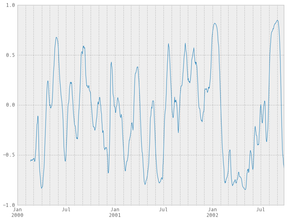
You can efficiently retrieve the time series of correlations between two columns using ix indexing:

In [231]: correls.ix[:, 'A', 'C'].plot()
Out[231]: <matplotlib.axes.AxesSubplot at 0x109f6a6d0>

Expanding window moment functions¶

A common alternative to rolling statistics is to use an expanding window, which yields the value of the statistic with all the data available up to that point in time. As these calculations are a special case of rolling statistics, they are implemented in pandas such that the following two calls are equivalent:

In [232]: rolling_mean(df, window=len(df), min_periods=1)[:5]
Out[232]: 
                   A         B         C         D
2000-01-01 -0.417884 -2.757922 -0.307713  0.150568
2000-01-02 -0.040474 -3.725653  0.196122  0.190333
2000-01-03 -0.401161 -4.246998  0.060725 -0.148770
2000-01-04 -0.797595 -4.788888  0.426269 -0.198859
2000-01-05 -0.978829 -5.523162  0.577954 -0.313535

In [233]: expanding_mean(df)[:5]
Out[233]: 
                   A         B         C         D
2000-01-01 -0.417884 -2.757922 -0.307713  0.150568
2000-01-02 -0.040474 -3.725653  0.196122  0.190333
2000-01-03 -0.401161 -4.246998  0.060725 -0.148770
2000-01-04 -0.797595 -4.788888  0.426269 -0.198859
2000-01-05 -0.978829 -5.523162  0.577954 -0.313535

Like the rolling_ functions, the following methods are included in the pandas namespace or can be located in pandas.stats.moments.

Function	Description
`expanding_count`	Number of non-null observations
`expanding_sum`	Sum of values
`expanding_mean`	Mean of values
`expanding_median`	Arithmetic median of values
`expanding_min`	Minimum
`expanding_max`	Maximum
`expanding_std`	Unbiased standard deviation
`expanding_var`	Unbiased variance
`expanding_skew`	Unbiased skewness (3rd moment)
`expanding_kurt`	Unbiased kurtosis (4th moment)
`expanding_quantile`	Sample quantile (value at %)
`expanding_apply`	Generic apply
`expanding_cov`	Unbiased covariance (binary)
`expanding_corr`	Correlation (binary)
`expanding_corr_pairwise`	Pairwise correlation of DataFrame columns

Aside from not having a window parameter, these functions have the same interfaces as their rolling_ counterpart. Like above, the parameters they all accept are:

min_periods: threshold of non-null data points to require. Defaults to minimum needed to compute statistic. No NaNs will be output once min_periods non-null data points have been seen.

freq: optionally specify a frequency string or DateOffset to pre-conform the data to. Note that prior to pandas v0.8.0, a keyword argument time_rule was used instead of freq that referred to the legacy time rule constants

Note

The output of the rolling_ and expanding_ functions do not return a NaN if there are at least min_periods non-null values in the current window. This differs from cumsum, cumprod, cummax, and cummin, which return NaN in the output wherever a NaN is encountered in the input.

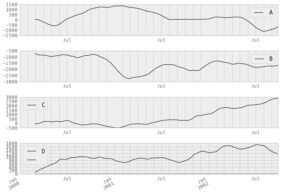
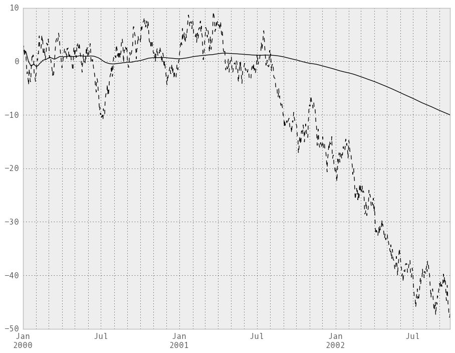
An expanding window statistic will be more stable (and less responsive) than its rolling window counterpart as the increasing window size decreases the relative impact of an individual data point. As an example, here is the expanding_mean output for the previous time series dataset:

In [234]: ts.plot(style='k--')
Out[234]: <matplotlib.axes.AxesSubplot at 0x1110083d0>

In [235]: expanding_mean(ts).plot(style='k')
Out[235]: <matplotlib.axes.AxesSubplot at 0x1110083d0>

Exponentially weighted moment functions¶

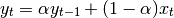
A related set of functions are exponentially weighted versions of many of the above statistics. A number of EW (exponentially weighted) functions are provided using the blending method. For example, where $y_t$ is the result and $x_t$ the input, we compute an exponentially weighted moving average as

$y_t = \alpha y_{t-1} + (1 - \alpha) x_t$

One must have $0 < \alpha \leq 1$ , but rather than pass $\alpha$ directly, it’s easier to think about either the span or center of mass (com) of an EW moment:

$\alpha = \begin{cases} \frac{2}{s + 1}, s = \text{span}\\ \frac{1}{c + 1}, c = \text{center of mass} \end{cases}$

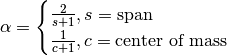
You can pass one or the other to these functions but not both. Span corresponds to what is commonly called a “20-day EW moving average” for example. Center of mass has a more physical interpretation. For example, span = 20 corresponds to com = 9.5. Here is the list of functions available:

Function	Description
`ewma`	EW moving average
`ewmvar`	EW moving variance
`ewmstd`	EW moving standard deviation
`ewmcorr`	EW moving correlation
`ewmcov`	EW moving covariance

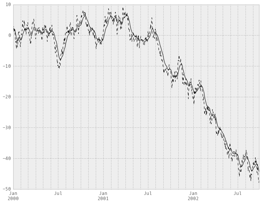
Here are an example for a univariate time series:

In [236]: plt.close('all')

In [237]: ts.plot(style='k--')
Out[237]: <matplotlib.axes.AxesSubplot at 0x111265a50>

In [238]: ewma(ts, span=20).plot(style='k')
Out[238]: <matplotlib.axes.AxesSubplot at 0x111265a50>

Note

The EW functions perform a standard adjustment to the initial observations whereby if there are fewer observations than called for in the span, those observations are reweighted accordingly.

Linear and panel regression¶

Note

We plan to move this functionality to statsmodels for the next release. Some of the result attributes may change names in order to foster naming consistency with the rest of statsmodels. We will provide every effort to provide compatibility with older versions of pandas, however.

We have implemented a very fast set of moving-window linear regression classes in pandas. Two different types of regressions are supported:

Standard ordinary least squares (OLS) multiple regression

Multiple regression (OLS-based) on panel data including with fixed-effects (also known as entity or individual effects) or time-effects.

Both kinds of linear models are accessed through the ols function in the pandas namespace. They all take the following arguments to specify either a static (full sample) or dynamic (moving window) regression:

window_type: 'full sample' (default), 'expanding', or rolling

window: size of the moving window in the window_type='rolling' case. If window is specified, window_type will be automatically set to 'rolling'

min_periods: minimum number of time periods to require to compute the regression coefficients

Generally speaking, the ols works by being given a y (response) object and an x (predictors) object. These can take many forms:

y: a Series, ndarray, or DataFrame (panel model)

x: Series, DataFrame, dict of Series, dict of DataFrame or Panel

Based on the types of y and x, the model will be inferred to either a panel model or a regular linear model. If the y variable is a DataFrame, the result will be a panel model. In this case, the x variable must either be a Panel, or a dict of DataFrame (which will be coerced into a Panel).

Standard OLS regression¶

Let’s pull in some sample data:

In [239]: from pandas.io.data import DataReader

In [240]: symbols = ['MSFT', 'GOOG', 'AAPL']

In [241]: data = dict((sym, DataReader(sym, "yahoo"))
   .....:             for sym in symbols)
   .....:

In [242]: panel = Panel(data).swapaxes('items', 'minor')

In [243]: close_px = panel['Close']

# convert closing prices to returns
In [244]: rets = close_px / close_px.shift(1) - 1

In [245]: rets.info()
<class 'pandas.core.frame.DataFrame'>
DatetimeIndex: 757 entries, 2010-01-04 00:00:00 to 2013-01-04 00:00:00
Data columns:
AAPL    756  non-null values
GOOG    756  non-null values
MSFT    756  non-null values
dtypes: float64(3)

Let’s do a static regression of AAPL returns on GOOG returns:

In [246]: model = ols(y=rets['AAPL'], x=rets.ix[:, ['GOOG']])

In [247]: model
Out[247]: 
-------------------------Summary of Regression Analysis-------------------------
Formula: Y ~ <GOOG> + <intercept>
Number of Observations:         756
Number of Degrees of Freedom:   2
R-squared:         0.2814
Adj R-squared:     0.2805
Rmse:              0.0147
F-stat (1, 754):   295.2873, p-value:     0.0000
Degrees of Freedom: model 1, resid 754
-----------------------Summary of Estimated Coefficients------------------------
      Variable       Coef    Std Err     t-stat    p-value    CI 2.5%   CI 97.5%
--------------------------------------------------------------------------------
          GOOG     0.5442     0.0317      17.18     0.0000     0.4822     0.6063
     intercept     0.0011     0.0005       2.14     0.0327     0.0001     0.0022
---------------------------------End of Summary---------------------------------

In [248]: model.beta
Out[248]: 
GOOG         0.544224
intercept    0.001147

If we had passed a Series instead of a DataFrame with the single GOOG column, the model would have assigned the generic name x to the sole right-hand side variable.

We can do a moving window regression to see how the relationship changes over time:

In [249]: model = ols(y=rets['AAPL'], x=rets.ix[:, ['GOOG']],
   .....:             window=250)
   .....:

# just plot the coefficient for GOOG
In [250]: model.beta['GOOG'].plot()
Out[250]: <matplotlib.axes.AxesSubplot at 0x10a6d77d0>

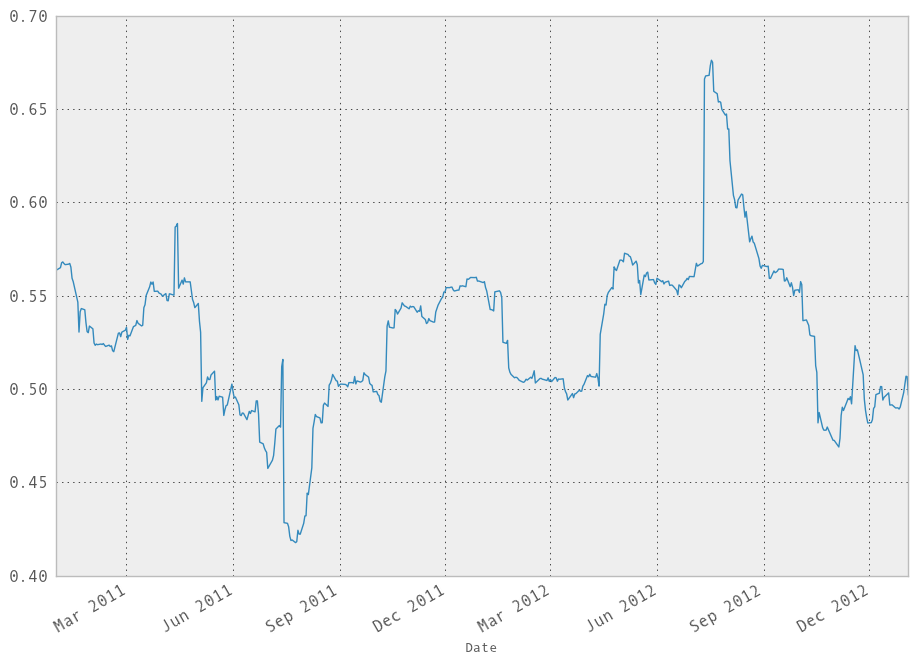
It looks like there are some outliers rolling in and out of the window in the above regression, influencing the results. We could perform a simple winsorization at the 3 STD level to trim the impact of outliers:

In [251]: winz = rets.copy()

In [252]: std_1year = rolling_std(rets, 250, min_periods=20)

# cap at 3 * 1 year standard deviation
In [253]: cap_level = 3 * np.sign(winz) * std_1year

In [254]: winz[np.abs(winz) > 3 * std_1year] = cap_level

In [255]: winz_model = ols(y=winz['AAPL'], x=winz.ix[:, ['GOOG']],
   .....:             window=250)
   .....:

In [256]: model.beta['GOOG'].plot(label="With outliers")
Out[256]: <matplotlib.axes.AxesSubplot at 0x10a6cd190>

In [257]: winz_model.beta['GOOG'].plot(label="Winsorized"); plt.legend(loc='best')
Out[257]: <matplotlib.legend.Legend at 0x111162b10>

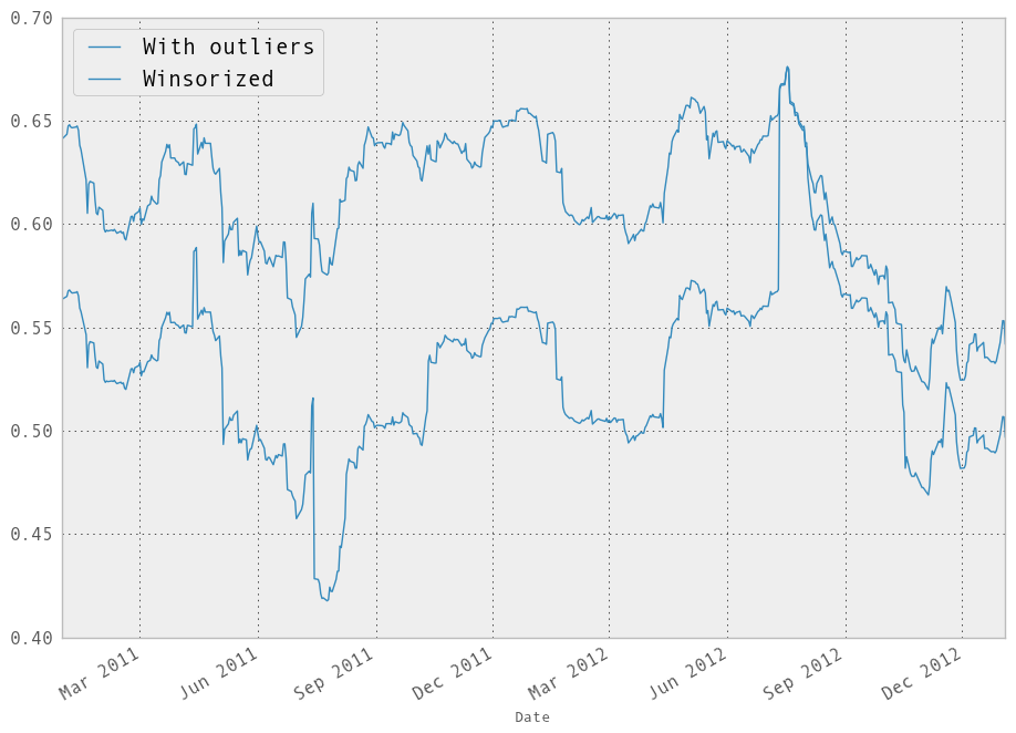
So in this simple example we see the impact of winsorization is actually quite significant. Note the correlation after winsorization remains high:

In [258]: winz.corrwith(rets)
Out[258]: 
AAPL    0.994969
GOOG    0.972473
MSFT    0.998387

Multiple regressions can be run by passing a DataFrame with multiple columns for the predictors x:

In [259]: ols(y=winz['AAPL'], x=winz.drop(['AAPL'], axis=1))
Out[259]: 
-------------------------Summary of Regression Analysis-------------------------
Formula: Y ~ <GOOG> + <MSFT> + <intercept>
Number of Observations:         756
Number of Degrees of Freedom:   3
R-squared:         0.3661
Adj R-squared:     0.3644
Rmse:              0.0133
F-stat (2, 753):   217.4516, p-value:     0.0000
Degrees of Freedom: model 2, resid 753
-----------------------Summary of Estimated Coefficients------------------------
      Variable       Coef    Std Err     t-stat    p-value    CI 2.5%   CI 97.5%
--------------------------------------------------------------------------------
          GOOG     0.4698     0.0373      12.58     0.0000     0.3967     0.5430
          MSFT     0.3164     0.0412       7.68     0.0000     0.2357     0.3972
     intercept     0.0011     0.0005       2.27     0.0235     0.0002     0.0021
---------------------------------End of Summary---------------------------------

Panel regression¶

We’ve implemented moving window panel regression on potentially unbalanced panel data (see this article if this means nothing to you). Suppose we wanted to model the relationship between the magnitude of the daily return and trading volume among a group of stocks, and we want to pool all the data together to run one big regression. This is actually quite easy:

# make the units somewhat comparable
In [260]: volume = panel['Volume'] / 1e8

In [261]: model = ols(y=volume, x={'return' : np.abs(rets)})

In [262]: model
Out[262]: 
-------------------------Summary of Regression Analysis-------------------------
Formula: Y ~ <return> + <intercept>
Number of Observations:         2268
Number of Degrees of Freedom:   2
R-squared:         0.0207
Adj R-squared:     0.0203
Rmse:              0.2683
F-stat (1, 2266):    47.9262, p-value:     0.0000
Degrees of Freedom: model 1, resid 2266
-----------------------Summary of Estimated Coefficients------------------------
      Variable       Coef    Std Err     t-stat    p-value    CI 2.5%   CI 97.5%
--------------------------------------------------------------------------------
        return     3.4632     0.5003       6.92     0.0000     2.4827     4.4437
     intercept     0.2247     0.0081      27.76     0.0000     0.2088     0.2406
---------------------------------End of Summary---------------------------------

In a panel model, we can insert dummy (0-1) variables for the “entities” involved (here, each of the stocks) to account the a entity-specific effect (intercept):

In [263]: fe_model = ols(y=volume, x={'return' : np.abs(rets)},
   .....:                entity_effects=True)
   .....:

In [264]: fe_model
Out[264]: 
-------------------------Summary of Regression Analysis-------------------------
Formula: Y ~ <return> + <FE_GOOG> + <FE_MSFT> + <intercept>
Number of Observations:         2268
Number of Degrees of Freedom:   4
R-squared:         0.7398
Adj R-squared:     0.7395
Rmse:              0.1383
F-stat (3, 2264):  2145.6389, p-value:     0.0000
Degrees of Freedom: model 3, resid 2264
-----------------------Summary of Estimated Coefficients------------------------
      Variable       Coef    Std Err     t-stat    p-value    CI 2.5%   CI 97.5%
--------------------------------------------------------------------------------
        return     4.5178     0.2589      17.45     0.0000     4.0103     5.0253
       FE_GOOG    -0.1568     0.0071     -22.01     0.0000    -0.1708    -0.1428
       FE_MSFT     0.3904     0.0071      54.67     0.0000     0.3764     0.4044
     intercept     0.1346     0.0060      22.29     0.0000     0.1227     0.1464
---------------------------------End of Summary---------------------------------

Because we ran the regression with an intercept, one of the dummy variables must be dropped or the design matrix will not be full rank. If we do not use an intercept, all of the dummy variables will be included:

In [265]: fe_model = ols(y=volume, x={'return' : np.abs(rets)},
   .....:                entity_effects=True, intercept=False)
   .....:

In [266]: fe_model
Out[266]: 
-------------------------Summary of Regression Analysis-------------------------
Formula: Y ~ <return> + <FE_AAPL> + <FE_GOOG> + <FE_MSFT>
Number of Observations:         2268
Number of Degrees of Freedom:   4
R-squared:         0.7398
Adj R-squared:     0.7395
Rmse:              0.1383
F-stat (4, 2264):  2145.6389, p-value:     0.0000
Degrees of Freedom: model 3, resid 2264
-----------------------Summary of Estimated Coefficients------------------------
      Variable       Coef    Std Err     t-stat    p-value    CI 2.5%   CI 97.5%
--------------------------------------------------------------------------------
        return     4.5178     0.2589      17.45     0.0000     4.0103     5.0253
       FE_AAPL     0.1346     0.0060      22.29     0.0000     0.1227     0.1464
       FE_GOOG    -0.0222     0.0058      -3.80     0.0001    -0.0337    -0.0108
       FE_MSFT     0.5250     0.0057      91.74     0.0000     0.5138     0.5362
---------------------------------End of Summary---------------------------------

We can also include time effects, which demeans the data cross-sectionally at each point in time (equivalent to including dummy variables for each date). More mathematical care must be taken to properly compute the standard errors in this case:

In [267]: te_model = ols(y=volume, x={'return' : np.abs(rets)},
   .....:                time_effects=True, entity_effects=True)
   .....:

In [268]: te_model
Out[268]: 
-------------------------Summary of Regression Analysis-------------------------
Formula: Y ~ <return> + <FE_GOOG> + <FE_MSFT>
Number of Observations:         2268
Number of Degrees of Freedom:   759
R-squared:         0.8165
Adj R-squared:     0.7243
Rmse:              0.1332
F-stat (3, 1509):     8.8584, p-value:     0.0000
Degrees of Freedom: model 758, resid 1509
-----------------------Summary of Estimated Coefficients------------------------
      Variable       Coef    Std Err     t-stat    p-value    CI 2.5%   CI 97.5%
--------------------------------------------------------------------------------
        return     3.7208     0.3739       9.95     0.0000     2.9880     4.4535
       FE_GOOG    -0.1579     0.0069     -22.98     0.0000    -0.1714    -0.1445
       FE_MSFT     0.3885     0.0069      56.25     0.0000     0.3750     0.4021
---------------------------------End of Summary---------------------------------

Here the intercept (the mean term) is dropped by default because it will be 0 according to the model assumptions, having subtracted off the group means.

Result fields and tests¶

We’ll leave it to the user to explore the docstrings and source, especially as we’ll be moving this code into statsmodels in the near future.

pandas 0.9.1 documentation

Table Of Contents

Search

Computational tools¶

Statistical functions¶

Percent Change¶

Covariance¶

Correlation¶

Data ranking¶

Moving (rolling) statistics / moments¶

Binary rolling moments¶

Computing rolling pairwise correlations¶

Expanding window moment functions¶

Exponentially weighted moment functions¶

Linear and panel regression¶

Standard OLS regression¶

Panel regression¶

Result fields and tests¶