Computational tools
Statistical functions
Percent Change
Both Series and DataFrame has a method pct_change to compute the percent change over a given number of periods (using fill_method to fill NA/null values).
In [209]: ser = Series(randn(8))

In [210]: ser.pct_change()
Out[210]:
0         NaN
1   -1.602976
2    4.334938
3   -0.247456
4   -2.067345
5   -1.142903
6   -1.688214
7   -9.759729
dtype: float64
In [211]: df = DataFrame(randn(10, 4))

In [212]: df.pct_change(periods=3)
Out[212]:
          0         1         2         3
0       NaN       NaN       NaN       NaN
1       NaN       NaN       NaN       NaN
2       NaN       NaN       NaN       NaN
3 -0.218320 -1.054001  1.987147 -0.510183
4 -0.439121 -1.816454  0.649715 -4.822809
5 -0.127833 -3.042065 -5.866604 -1.776977
6 -2.596833 -1.959538 -2.111697 -3.798900
7 -0.117826 -2.169058  0.036094 -0.067696
8  2.492606 -1.357320 -1.205802 -1.558697
9 -1.012977  2.324558 -1.003744 -0.371806
Covariance
The Series object has a method cov to compute covariance between series (excluding NA/null values).
In [213]: s1 = Series(randn(1000))

In [214]: s2 = Series(randn(1000))

In [215]: s1.cov(s2)
Out[215]: 0.00068010881743109321
Analogously, DataFrame has a method cov to compute pairwise covariances among the series in the DataFrame, also excluding NA/null values.
In [216]: frame = DataFrame(randn(1000, 5), columns=['a', 'b', 'c', 'd', 'e'])

In [217]: frame.cov()
Out[217]:
          a         b         c         d         e
a  1.000882 -0.003177 -0.002698 -0.006889  0.031912
b -0.003177  1.024721  0.000191  0.009212  0.000857
c -0.002698  0.000191  0.950735 -0.031743 -0.005087
d -0.006889  0.009212 -0.031743  1.002983 -0.047952
e  0.031912  0.000857 -0.005087 -0.047952  1.042487
DataFrame.cov also supports an optional min_periods keyword that specifies the required minimum number of observations for each column pair in order to have a valid result.
In [218]: frame = DataFrame(randn(20, 3), columns=['a', 'b', 'c'])

In [219]: frame.ix[:5, 'a'] = np.nan

In [220]: frame.ix[5:10, 'b'] = np.nan

In [221]: frame.cov()
Out[221]:
          a         b         c
a  1.210090 -0.430629  0.018002
b -0.430629  1.240960  0.347188
c  0.018002  0.347188  1.301149

In [222]: frame.cov(min_periods=12)
Out[222]:
          a         b         c
a  1.210090       NaN  0.018002
b       NaN  1.240960  0.347188
c  0.018002  0.347188  1.301149
Correlation
Several methods for computing correlations are provided. Several kinds of correlation methods are provided:
| Method name | Description |
|---|---|
| pearson (default) | Standard correlation coefficient |
| kendall | Kendall Tau correlation coefficient |
| spearman | Spearman rank correlation coefficient |
All of these are currently computed using pairwise complete observations.
In [223]: frame = DataFrame(randn(1000, 5), columns=['a', 'b', 'c', 'd', 'e'])

In [224]: frame.ix[::2] = np.nan

# Series with Series
In [225]: frame['a'].corr(frame['b'])
Out[225]: 0.013479040400098763

In [226]: frame['a'].corr(frame['b'], method='spearman')
Out[226]: -0.0072898851595406388

# Pairwise correlation of DataFrame columns
In [227]: frame.corr()
Out[227]:
          a         b         c         d         e
a  1.000000  0.013479 -0.049269 -0.042239 -0.028525
b  0.013479  1.000000 -0.020433 -0.011139  0.005654
c -0.049269 -0.020433  1.000000  0.018587 -0.054269
d -0.042239 -0.011139  0.018587  1.000000 -0.017060
e -0.028525  0.005654 -0.054269 -0.017060  1.000000
Note that non-numeric columns will be automatically excluded from the correlation calculation.
Like cov, corr also supports the optional min_periods keyword:
In [228]: frame = DataFrame(randn(20, 3), columns=['a', 'b', 'c'])

In [229]: frame.ix[:5, 'a'] = np.nan

In [230]: frame.ix[5:10, 'b'] = np.nan

In [231]: frame.corr()
Out[231]:
          a         b         c
a  1.000000 -0.076520  0.160092
b -0.076520  1.000000  0.135967
c  0.160092  0.135967  1.000000

In [232]: frame.corr(min_periods=12)
Out[232]:
          a         b         c
a  1.000000       NaN  0.160092
b       NaN  1.000000  0.135967
c  0.160092  0.135967  1.000000
A related method corrwith is implemented on DataFrame to compute the correlation between like-labeled Series contained in different DataFrame objects.
In [233]: index = ['a', 'b', 'c', 'd', 'e']

In [234]: columns = ['one', 'two', 'three', 'four']

In [235]: df1 = DataFrame(randn(5, 4), index=index, columns=columns)

In [236]: df2 = DataFrame(randn(4, 4), index=index[:4], columns=columns)

In [237]: df1.corrwith(df2)
Out[237]:
one     -0.125501
two     -0.493244
three    0.344056
four     0.004183
dtype: float64

In [238]: df2.corrwith(df1, axis=1)
Out[238]:
a   -0.675817
b    0.458296
c    0.190809
d   -0.186275
e         NaN
dtype: float64
Data ranking
The rank method produces a data ranking with ties being assigned the mean of the ranks (by default) for the group:
In [239]: s = Series(np.random.randn(5), index=list('abcde'))

In [240]: s['d'] = s['b'] # so there's a tie

In [241]: s.rank()
Out[241]:
a    5.0
b    2.5
c    1.0
d    2.5
e    4.0
dtype: float64
rank is also a DataFrame method and can rank either the rows (axis=0) or the columns (axis=1). NaN values are excluded from the ranking.
In [242]: df = DataFrame(np.random.randn(10, 6))

In [243]: df[4] = df[2][:5] # some ties

In [244]: df
Out[244]:
          0         1         2         3         4         5
0 -0.904948 -1.163537 -1.457187  0.135463 -1.457187  0.294650
1 -0.976288 -0.244652 -0.748406 -0.999601 -0.748406 -0.800809
2  0.401965  1.460840  1.256057  1.308127  1.256057  0.876004
3  0.205954  0.369552 -0.669304  0.038378 -0.669304  1.140296
4 -0.477586 -0.730705 -1.129149 -0.601463 -1.129149 -0.211196
5 -1.092970 -0.689246  0.908114  0.204848       NaN  0.463347
6  0.376892  0.959292  0.095572 -0.593740       NaN -0.069180
7 -1.002601  1.957794 -0.120708  0.094214       NaN -1.467422
8 -0.547231  0.664402 -0.519424 -0.073254       NaN -1.263544
9 -0.250277 -0.237428 -1.056443  0.419477       NaN  1.375064

In [245]: df.rank(1)
Out[245]:
   0  1    2  3    4  5
0  4  3  1.5  5  1.5  6
1  2  6  4.5  1  4.5  3
2  1  6  3.5  5  3.5  2
3  4  5  1.5  3  1.5  6
4  5  3  1.5  4  1.5  6
5  1  2  5.0  3  NaN  4
6  4  5  3.0  1  NaN  2
7  2  5  3.0  4  NaN  1
8  2  5  3.0  4  NaN  1
9  2  3  1.0  4  NaN  5
rank optionally takes a parameter ascending which by default is true; when false, data is reverse-ranked, with larger values assigned a smaller rank.
rank supports different tie-breaking methods, specified with the method parameter:
- average : average rank of tied group
- min : lowest rank in the group
- max : highest rank in the group
- first : ranks assigned in the order they appear in the array
Note
These methods are significantly faster (around 10-20x) than scipy.stats.rankdata.
Moving (rolling) statistics / moments
For working with time series data, a number of functions are provided for computing common moving or rolling statistics. Among these are count, sum, mean, median, correlation, variance, covariance, standard deviation, skewness, and kurtosis. All of these methods are in the pandas namespace, but otherwise they can be found in pandas.stats.moments.
| Function | Description |
|---|---|
| rolling_count | Number of non-null observations |
| rolling_sum | Sum of values |
| rolling_mean | Mean of values |
| rolling_median | Arithmetic median of values |
| rolling_min | Minimum |
| rolling_max | Maximum |
| rolling_std | Unbiased standard deviation |
| rolling_var | Unbiased variance |
| rolling_skew | Unbiased skewness (3rd moment) |
| rolling_kurt | Unbiased kurtosis (4th moment) |
| rolling_quantile | Sample quantile (value at %) |
| rolling_apply | Generic apply |
| rolling_cov | Unbiased covariance (binary) |
| rolling_corr | Correlation (binary) |
| rolling_corr_pairwise | Pairwise correlation of DataFrame columns |
| rolling_window | Moving window function |
Generally these methods all have the same interface. The binary operators (e.g. rolling_corr) take two Series or DataFrames. Otherwise, they all accept the following arguments:
- window: size of moving window
- min_periods: threshold of non-null data points to require (otherwise result is NA)
- freq: optionally specify a frequency string or DateOffset to pre-conform the data to. Note that prior to pandas v0.8.0, a keyword argument time_rule was used instead of freq that referred to the legacy time rule constants
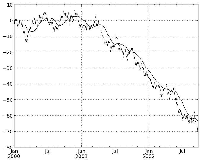
These functions can be applied to ndarrays or Series objects:
In [246]: ts = Series(randn(1000), index=date_range('1/1/2000', periods=1000))

In [247]: ts = ts.cumsum()

In [248]: ts.plot(style='k--')
Out[248]: <matplotlib.axes.AxesSubplot at 0x6691590>

In [249]: rolling_mean(ts, 60).plot(style='k')
Out[249]: <matplotlib.axes.AxesSubplot at 0x6691590>
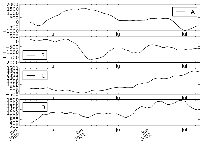
They can also be applied to DataFrame objects. This is really just syntactic sugar for applying the moving window operator to all of the DataFrame’s columns:
In [250]: df = DataFrame(randn(1000, 4), index=ts.index,
   .....:                columns=['A', 'B', 'C', 'D'])
   .....:

In [251]: df = df.cumsum()

In [252]: rolling_sum(df, 60).plot(subplots=True)
Out[252]:
array([Axes(0.125,0.747826;0.775x0.152174),
       Axes(0.125,0.565217;0.775x0.152174),
       Axes(0.125,0.382609;0.775x0.152174), Axes(0.125,0.2;0.775x0.152174)], dtype=object)
The rolling_apply function takes an extra func argument and performs generic rolling computations. The func argument should be a single function that produces a single value from an ndarray input. Suppose we wanted to compute the mean absolute deviation on a rolling basis:
In [253]: mad = lambda x: np.fabs(x - x.mean()).mean()

In [254]: rolling_apply(ts, 60, mad).plot(style='k')
Out[254]: <matplotlib.axes.AxesSubplot at 0x6d4f750>
The rolling_window function performs a generic rolling window computation on the input data. The weights used in the window are specified by the win_type keyword. The list of recognized types are:
- boxcar
- triang
- blackman
- hamming
- bartlett
- parzen
- bohman
- blackmanharris
- nuttall
- barthann
- kaiser (needs beta)
- gaussian (needs std)
- general_gaussian (needs power, width)
- slepian (needs width).
In [255]: ser = Series(randn(10), index=date_range('1/1/2000', periods=10))

In [256]: rolling_window(ser, 5, 'triang')
Out[256]:
2000-01-01         NaN
2000-01-02         NaN
2000-01-03         NaN
2000-01-04         NaN
2000-01-05   -0.622722
2000-01-06   -0.460623
2000-01-07   -0.229918
2000-01-08   -0.237308
2000-01-09   -0.335064
2000-01-10   -0.403449
Freq: D, dtype: float64
Note that the boxcar window is equivalent to rolling_mean:
In [257]: rolling_window(ser, 5, 'boxcar')
Out[257]:
2000-01-01         NaN
2000-01-02         NaN
2000-01-03         NaN
2000-01-04         NaN
2000-01-05   -0.841164
2000-01-06   -0.779948
2000-01-07   -0.565487
2000-01-08   -0.502815
2000-01-09   -0.553755
2000-01-10   -0.472211
Freq: D, dtype: float64

In [258]: rolling_mean(ser, 5)
Out[258]:
2000-01-01         NaN
2000-01-02         NaN
2000-01-03         NaN
2000-01-04         NaN
2000-01-05   -0.841164
2000-01-06   -0.779948
2000-01-07   -0.565487
2000-01-08   -0.502815
2000-01-09   -0.553755
2000-01-10   -0.472211
Freq: D, dtype: float64
For some windowing functions, additional parameters must be specified:
In [259]: rolling_window(ser, 5, 'gaussian', std=0.1)
Out[259]:
2000-01-01         NaN
2000-01-02         NaN
2000-01-03         NaN
2000-01-04         NaN
2000-01-05   -0.261998
2000-01-06   -0.230600
2000-01-07    0.121276
2000-01-08   -0.136220
2000-01-09   -0.057945
2000-01-10   -0.199326
Freq: D, dtype: float64
By default the labels are set to the right edge of the window, but a center keyword is available so the labels can be set at the center. This keyword is available in other rolling functions as well.
In [260]: rolling_window(ser, 5, 'boxcar')
Out[260]:
2000-01-01         NaN
2000-01-02         NaN
2000-01-03         NaN
2000-01-04         NaN
2000-01-05   -0.841164
2000-01-06   -0.779948
2000-01-07   -0.565487
2000-01-08   -0.502815
2000-01-09   -0.553755
2000-01-10   -0.472211
Freq: D, dtype: float64

In [261]: rolling_window(ser, 5, 'boxcar', center=True)
Out[261]:
2000-01-01         NaN
2000-01-02         NaN
2000-01-03   -0.841164
2000-01-04   -0.779948
2000-01-05   -0.565487
2000-01-06   -0.502815
2000-01-07   -0.553755
2000-01-08   -0.472211
2000-01-09         NaN
2000-01-10         NaN
Freq: D, dtype: float64

In [262]: rolling_mean(ser, 5, center=True)
Out[262]:
2000-01-01         NaN
2000-01-02         NaN
2000-01-03   -0.841164
2000-01-04   -0.779948
2000-01-05   -0.565487
2000-01-06   -0.502815
2000-01-07   -0.553755
2000-01-08   -0.472211
2000-01-09         NaN
2000-01-10         NaN
Freq: D, dtype: float64
Binary rolling moments
rolling_cov and rolling_corr can compute moving window statistics about two Series or any combination of DataFrame/Series or DataFrame/DataFrame. Here is the behavior in each case:
- two Series: compute the statistic for the pairing
- DataFrame/Series: compute the statistics for each column of the DataFrame with the passed Series, thus returning a DataFrame
- DataFrame/DataFrame: compute statistic for matching column names, returning a DataFrame
For example:
In [263]: df2 = df[:20]

In [264]: rolling_corr(df2, df2['B'], window=5)
Out[264]:
                   A   B         C         D
2000-01-01       NaN NaN       NaN       NaN
2000-01-02       NaN NaN       NaN       NaN
2000-01-03       NaN NaN       NaN       NaN
2000-01-04       NaN NaN       NaN       NaN
2000-01-05 -0.262853   1  0.334449  0.193380
2000-01-06 -0.083745   1 -0.521587 -0.556126
2000-01-07 -0.292940   1 -0.658532 -0.458128
2000-01-08  0.840416   1  0.796505 -0.498672
2000-01-09 -0.135275   1  0.753895 -0.634445
2000-01-10 -0.346229   1 -0.682232 -0.645681
2000-01-11 -0.365524   1 -0.775831 -0.561991
2000-01-12 -0.204761   1 -0.855874 -0.382232
2000-01-13  0.575218   1 -0.747531  0.167892
2000-01-14  0.519499   1 -0.687277  0.192822
2000-01-15  0.048982   1  0.167669 -0.061463
2000-01-16  0.217190   1  0.167564 -0.326034
2000-01-17  0.641180   1 -0.164780 -0.111487
2000-01-18  0.130422   1  0.322833  0.632383
2000-01-19  0.317278   1  0.384528  0.813656
2000-01-20  0.293598   1  0.159538  0.742381
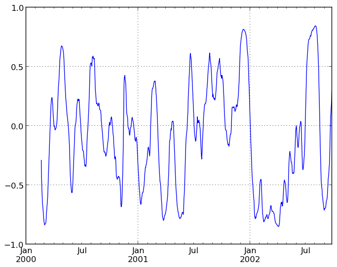
Computing rolling pairwise correlations
In financial data analysis and other fields it’s common to compute correlation matrices for a collection of time series. More difficult is to compute a moving-window correlation matrix. This can be done using the rolling_corr_pairwise function, which yields a Panel whose items are the dates in question:
In [265]: correls = rolling_corr_pairwise(df, 50)

In [266]: correls[df.index[-50]]
Out[266]:
          A         B         C         D
A  1.000000  0.604221  0.767429 -0.776170
B  0.604221  1.000000  0.461484 -0.381148
C  0.767429  0.461484  1.000000 -0.748863
D -0.776170 -0.381148 -0.748863  1.000000
You can efficiently retrieve the time series of correlations between two columns using ix indexing:
In [267]: correls.ix[:, 'A', 'C'].plot()
Out[267]: <matplotlib.axes.AxesSubplot at 0x6d76590>
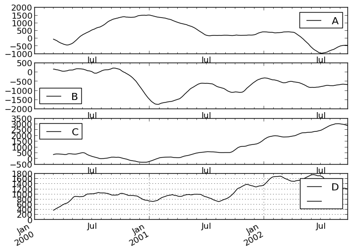
Expanding window moment functions
A common alternative to rolling statistics is to use an expanding window, which yields the value of the statistic with all the data available up to that point in time. As these calculations are a special case of rolling statistics, they are implemented in pandas such that the following two calls are equivalent:
In [268]: rolling_mean(df, window=len(df), min_periods=1)[:5]
Out[268]:
                   A         B         C         D
2000-01-01 -1.388345  3.317290  0.344542 -0.036968
2000-01-02 -1.123132  3.622300  1.675867  0.595300
2000-01-03 -0.628502  3.626503  2.455240  1.060158
2000-01-04 -0.768740  3.888917  2.451354  1.281874
2000-01-05 -0.824034  4.108035  2.556112  1.140723

In [269]: expanding_mean(df)[:5]
Out[269]:
                   A         B         C         D
2000-01-01 -1.388345  3.317290  0.344542 -0.036968
2000-01-02 -1.123132  3.622300  1.675867  0.595300
2000-01-03 -0.628502  3.626503  2.455240  1.060158
2000-01-04 -0.768740  3.888917  2.451354  1.281874
2000-01-05 -0.824034  4.108035  2.556112  1.140723
Like the rolling_ functions, the following methods are included in the pandas namespace or can be located in pandas.stats.moments.
| Function | Description |
|---|---|
| expanding_count | Number of non-null observations |
| expanding_sum | Sum of values |
| expanding_mean | Mean of values |
| expanding_median | Arithmetic median of values |
| expanding_min | Minimum |
| expanding_max | Maximum |
| expanding_std | Unbiased standard deviation |
| expanding_var | Unbiased variance |
| expanding_skew | Unbiased skewness (3rd moment) |
| expanding_kurt | Unbiased kurtosis (4th moment) |
| expanding_quantile | Sample quantile (value at %) |
| expanding_apply | Generic apply |
| expanding_cov | Unbiased covariance (binary) |
| expanding_corr | Correlation (binary) |
| expanding_corr_pairwise | Pairwise correlation of DataFrame columns |
Aside from not having a window parameter, these functions have the same interfaces as their rolling_ counterpart. Like above, the parameters they all accept are:
- min_periods: threshold of non-null data points to require. Defaults to minimum needed to compute statistic. No NaNs will be output once min_periods non-null data points have been seen.
- freq: optionally specify a frequency string or DateOffset to pre-conform the data to. Note that prior to pandas v0.8.0, a keyword argument time_rule was used instead of freq that referred to the legacy time rule constants
Note
The output of the rolling_ and expanding_ functions do not return a NaN if there are at least min_periods non-null values in the current window. This differs from cumsum, cumprod, cummax, and cummin, which return NaN in the output wherever a NaN is encountered in the input.
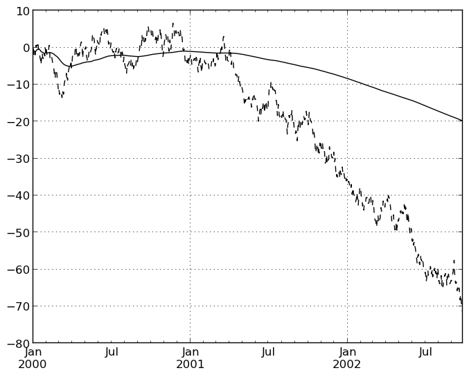
An expanding window statistic will be more stable (and less responsive) than its rolling window counterpart as the increasing window size decreases the relative impact of an individual data point. As an example, here is the expanding_mean output for the previous time series dataset:
In [270]: ts.plot(style='k--')
Out[270]: <matplotlib.axes.AxesSubplot at 0x74323d0>

In [271]: expanding_mean(ts).plot(style='k')
Out[271]: <matplotlib.axes.AxesSubplot at 0x74323d0>
Exponentially weighted moment functions
A related set of functions are exponentially weighted versions of many of the
above statistics. A number of EW (exponentially weighted) functions are
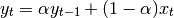
provided using the blending method. For example, where  is the
result and
is the
result and  the input, we compute an exponentially weighted moving
average as
the input, we compute an exponentially weighted moving
average as
One must have  , but rather than pass
  directly, it’s easier to think about either the span or center of mass
(com) of an EW moment:
directly, it’s easier to think about either the span or center of mass
(com) of an EW moment:
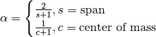
You can pass one or the other to these functions but not both. Span corresponds to what is commonly called a “20-day EW moving average” for example. Center of mass has a more physical interpretation. For example, span = 20 corresponds to com = 9.5. Here is the list of functions available:
| Function | Description |
|---|---|
| ewma | EW moving average |
| ewmvar | EW moving variance |
| ewmstd | EW moving standard deviation |
| ewmcorr | EW moving correlation |
| ewmcov | EW moving covariance |
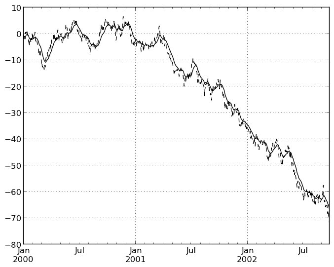
Here are an example for a univariate time series:
In [272]: plt.close('all')

In [273]: ts.plot(style='k--')
Out[273]: <matplotlib.axes.AxesSubplot at 0x77b2950>

In [274]: ewma(ts, span=20).plot(style='k')
Out[274]: <matplotlib.axes.AxesSubplot at 0x77b2950>
Note
The EW functions perform a standard adjustment to the initial observations whereby if there are fewer observations than called for in the span, those observations are reweighted accordingly.
Linear and panel regression
Note
We plan to move this functionality to statsmodels for the next release. Some of the result attributes may change names in order to foster naming consistency with the rest of statsmodels. We will provide every effort to provide compatibility with older versions of pandas, however.
We have implemented a very fast set of moving-window linear regression classes in pandas. Two different types of regressions are supported:
- Standard ordinary least squares (OLS) multiple regression
- Multiple regression (OLS-based) on panel data including with fixed-effects (also known as entity or individual effects) or time-effects.
Both kinds of linear models are accessed through the ols function in the pandas namespace. They all take the following arguments to specify either a static (full sample) or dynamic (moving window) regression:
- window_type: 'full sample' (default), 'expanding', or rolling
- window: size of the moving window in the window_type='rolling' case. If window is specified, window_type will be automatically set to 'rolling'
- min_periods: minimum number of time periods to require to compute the regression coefficients
Generally speaking, the ols works by being given a y (response) object and an x (predictors) object. These can take many forms:
- y: a Series, ndarray, or DataFrame (panel model)
- x: Series, DataFrame, dict of Series, dict of DataFrame or Panel
Based on the types of y and x, the model will be inferred to either a panel model or a regular linear model. If the y variable is a DataFrame, the result will be a panel model. In this case, the x variable must either be a Panel, or a dict of DataFrame (which will be coerced into a Panel).
Standard OLS regression
Let’s pull in some sample data:
In [275]: from pandas.io.data import DataReader

In [276]: symbols = ['MSFT', 'GOOG', 'AAPL']

In [277]: data = dict((sym, DataReader(sym, "yahoo"))
   .....:             for sym in symbols)
   .....:

In [278]: panel = Panel(data).swapaxes('items', 'minor')

In [279]: close_px = panel['Close']

# convert closing prices to returns
In [280]: rets = close_px / close_px.shift(1) - 1

In [281]: rets.info()
<class 'pandas.core.frame.DataFrame'>
DatetimeIndex: 830 entries, 2010-01-04 00:00:00 to 2013-04-22 00:00:00
Data columns:
AAPL    829  non-null values
GOOG    829  non-null values
MSFT    829  non-null values
dtypes: float64(3)
Let’s do a static regression of AAPL returns on GOOG returns:
In [282]: model = ols(y=rets['AAPL'], x=rets.ix[:, ['GOOG']])

In [283]: model
Out[283]:
-------------------------Summary of Regression Analysis-------------------------
Formula: Y ~ <GOOG> + <intercept>
Number of Observations:         829
Number of Degrees of Freedom:   2
R-squared:         0.2372
Adj R-squared:     0.2363
Rmse:              0.0157
F-stat (1, 827):   257.2205, p-value:     0.0000
Degrees of Freedom: model 1, resid 827
-----------------------Summary of Estimated Coefficients------------------------
      Variable       Coef    Std Err     t-stat    p-value    CI 2.5%   CI 97.5%
--------------------------------------------------------------------------------
          GOOG     0.5267     0.0328      16.04     0.0000     0.4623     0.5910
     intercept     0.0007     0.0005       1.25     0.2101    -0.0004     0.0018
---------------------------------End of Summary---------------------------------

In [284]: model.beta
Out[284]:
GOOG         0.526664
intercept    0.000685
dtype: float64
If we had passed a Series instead of a DataFrame with the single GOOG column, the model would have assigned the generic name x to the sole right-hand side variable.
We can do a moving window regression to see how the relationship changes over time:
In [285]: model = ols(y=rets['AAPL'], x=rets.ix[:, ['GOOG']],
   .....:             window=250)
   .....:

# just plot the coefficient for GOOG
In [286]: model.beta['GOOG'].plot()
Out[286]: <matplotlib.axes.AxesSubplot at 0x8160410>
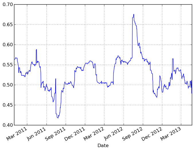
It looks like there are some outliers rolling in and out of the window in the above regression, influencing the results. We could perform a simple winsorization at the 3 STD level to trim the impact of outliers:
In [287]: winz = rets.copy()

In [288]: std_1year = rolling_std(rets, 250, min_periods=20)

# cap at 3 * 1 year standard deviation
In [289]: cap_level = 3 * np.sign(winz) * std_1year

In [290]: winz[np.abs(winz) > 3 * std_1year] = cap_level

In [291]: winz_model = ols(y=winz['AAPL'], x=winz.ix[:, ['GOOG']],
   .....:             window=250)
   .....:

In [292]: model.beta['GOOG'].plot(label="With outliers")
Out[292]: <matplotlib.axes.AxesSubplot at 0x8d91dd0>

In [293]: winz_model.beta['GOOG'].plot(label="Winsorized"); plt.legend(loc='best')
Out[293]: <matplotlib.legend.Legend at 0x8eb97d0>
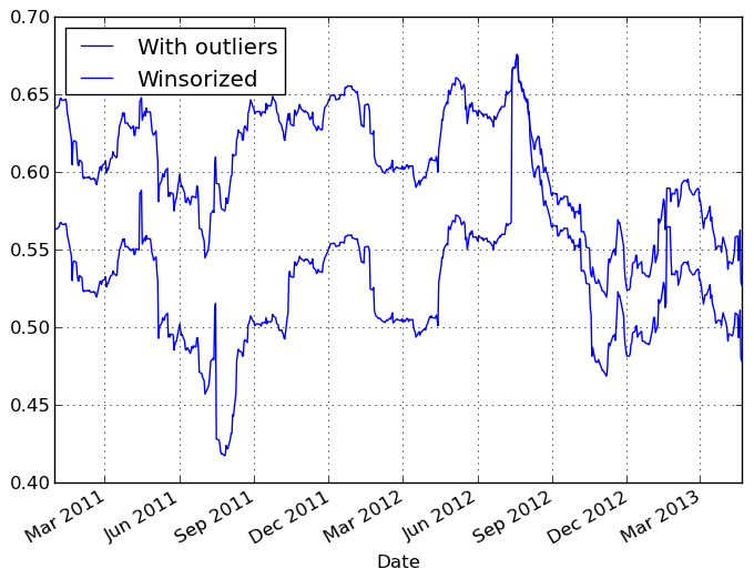
So in this simple example we see the impact of winsorization is actually quite significant. Note the correlation after winsorization remains high:
In [294]: winz.corrwith(rets)
Out[294]:
AAPL    0.988868
GOOG    0.973599
MSFT    0.998398
dtype: float64
Multiple regressions can be run by passing a DataFrame with multiple columns for the predictors x:
In [295]: ols(y=winz['AAPL'], x=winz.drop(['AAPL'], axis=1))
Out[295]:
-------------------------Summary of Regression Analysis-------------------------
Formula: Y ~ <GOOG> + <MSFT> + <intercept>
Number of Observations:         829
Number of Degrees of Freedom:   3
R-squared:         0.3217
Adj R-squared:     0.3200
Rmse:              0.0140
F-stat (2, 826):   195.8485, p-value:     0.0000
Degrees of Freedom: model 2, resid 826
-----------------------Summary of Estimated Coefficients------------------------
      Variable       Coef    Std Err     t-stat    p-value    CI 2.5%   CI 97.5%
--------------------------------------------------------------------------------
          GOOG     0.4636     0.0380      12.20     0.0000     0.3892     0.5381
          MSFT     0.2956     0.0418       7.07     0.0000     0.2136     0.3777
     intercept     0.0007     0.0005       1.38     0.1666    -0.0003     0.0016
---------------------------------End of Summary---------------------------------
Panel regression
We’ve implemented moving window panel regression on potentially unbalanced panel data (see this article if this means nothing to you). Suppose we wanted to model the relationship between the magnitude of the daily return and trading volume among a group of stocks, and we want to pool all the data together to run one big regression. This is actually quite easy:
# make the units somewhat comparable
In [296]: volume = panel['Volume'] / 1e8

In [297]: model = ols(y=volume, x={'return' : np.abs(rets)})

In [298]: model
Out[298]:
-------------------------Summary of Regression Analysis-------------------------
Formula: Y ~ <return> + <intercept>
Number of Observations:         2487
Number of Degrees of Freedom:   2
R-squared:         0.0211
Adj R-squared:     0.0207
Rmse:              0.2654
F-stat (1, 2485):    53.6545, p-value:     0.0000
Degrees of Freedom: model 1, resid 2485
-----------------------Summary of Estimated Coefficients------------------------
      Variable       Coef    Std Err     t-stat    p-value    CI 2.5%   CI 97.5%
--------------------------------------------------------------------------------
        return     3.4208     0.4670       7.32     0.0000     2.5055     4.3362
     intercept     0.2227     0.0076      29.38     0.0000     0.2079     0.2376
---------------------------------End of Summary---------------------------------
In a panel model, we can insert dummy (0-1) variables for the “entities” involved (here, each of the stocks) to account the a entity-specific effect (intercept):
In [299]: fe_model = ols(y=volume, x={'return' : np.abs(rets)},
   .....:                entity_effects=True)
   .....:

In [300]: fe_model
Out[300]:
-------------------------Summary of Regression Analysis-------------------------
Formula: Y ~ <return> + <FE_GOOG> + <FE_MSFT> + <intercept>
Number of Observations:         2487
Number of Degrees of Freedom:   4
R-squared:         0.7401
Adj R-squared:     0.7398
Rmse:              0.1368
F-stat (3, 2483):  2357.1701, p-value:     0.0000
Degrees of Freedom: model 3, resid 2483
-----------------------Summary of Estimated Coefficients------------------------
      Variable       Coef    Std Err     t-stat    p-value    CI 2.5%   CI 97.5%
--------------------------------------------------------------------------------
        return     4.5616     0.2420      18.85     0.0000     4.0872     5.0360
       FE_GOOG    -0.1540     0.0067     -22.87     0.0000    -0.1672    -0.1408
       FE_MSFT     0.3873     0.0068      57.34     0.0000     0.3741     0.4006
     intercept     0.1318     0.0057      23.04     0.0000     0.1206     0.1430
---------------------------------End of Summary---------------------------------
Because we ran the regression with an intercept, one of the dummy variables must be dropped or the design matrix will not be full rank. If we do not use an intercept, all of the dummy variables will be included:
In [301]: fe_model = ols(y=volume, x={'return' : np.abs(rets)},
   .....:                entity_effects=True, intercept=False)
   .....:

In [302]: fe_model
Out[302]:
-------------------------Summary of Regression Analysis-------------------------
Formula: Y ~ <return> + <FE_AAPL> + <FE_GOOG> + <FE_MSFT>
Number of Observations:         2487
Number of Degrees of Freedom:   4
R-squared:         0.7401
Adj R-squared:     0.7398
Rmse:              0.1368
F-stat (4, 2483):  2357.1701, p-value:     0.0000
Degrees of Freedom: model 3, resid 2483
-----------------------Summary of Estimated Coefficients------------------------
      Variable       Coef    Std Err     t-stat    p-value    CI 2.5%   CI 97.5%
--------------------------------------------------------------------------------
        return     4.5616     0.2420      18.85     0.0000     4.0872     5.0360
       FE_AAPL     0.1318     0.0057      23.04     0.0000     0.1206     0.1430
       FE_GOOG    -0.0223     0.0055      -4.07     0.0000    -0.0330    -0.0115
       FE_MSFT     0.5191     0.0054      96.76     0.0000     0.5086     0.5296
---------------------------------End of Summary---------------------------------
We can also include time effects, which demeans the data cross-sectionally at each point in time (equivalent to including dummy variables for each date). More mathematical care must be taken to properly compute the standard errors in this case:
In [303]: te_model = ols(y=volume, x={'return' : np.abs(rets)},
   .....:                time_effects=True, entity_effects=True)
   .....:

In [304]: te_model
Out[304]:
-------------------------Summary of Regression Analysis-------------------------
Formula: Y ~ <return> + <FE_GOOG> + <FE_MSFT>
Number of Observations:         2487
Number of Degrees of Freedom:   832
R-squared:         0.8159
Adj R-squared:     0.7235
Rmse:              0.1320
F-stat (3, 1655):     8.8284, p-value:     0.0000
Degrees of Freedom: model 831, resid 1655
-----------------------Summary of Estimated Coefficients------------------------
      Variable       Coef    Std Err     t-stat    p-value    CI 2.5%   CI 97.5%
--------------------------------------------------------------------------------
        return     3.7304     0.3422      10.90     0.0000     3.0597     4.4011
       FE_GOOG    -0.1556     0.0065     -23.89     0.0000    -0.1684    -0.1428
       FE_MSFT     0.3850     0.0066      58.72     0.0000     0.3721     0.3978
---------------------------------End of Summary---------------------------------
Here the intercept (the mean term) is dropped by default because it will be 0 according to the model assumptions, having subtracted off the group means.
Result fields and tests
We’ll leave it to the user to explore the docstrings and source, especially as we’ll be moving this code into statsmodels in the near future.