Indexing and Selecting Data
The axis labeling information in pandas objects serves many purposes:
- Identifies data (i.e. provides metadata) using known indicators, important for analysis, visualization, and interactive console display
- Enables automatic and explicit data alignment
- Allows intuitive getting and setting of subsets of the data set
In this section, we will focus on the final point: namely, how to slice, dice, and generally get and set subsets of pandas objects. The primary focus will be on Series and DataFrame as they have received more development attention in this area. Expect more work to be invested higher-dimensional data structures (including Panel) in the future, especially in label-based advanced indexing.
Note
The Python and NumPy indexing operators [] and attribute operator . provide quick and easy access to pandas data structures across a wide range of use cases. This makes interactive work intuitive, as there’s little new to learn if you already know how to deal with Python dictionaries and NumPy arrays. However, since the type of the data to be accessed isn’t known in advance, directly using standard operators has some optimization limits. For production code, we recommended that you take advantage of the optimized pandas data access methods exposed in this chapter.
Warning
Whether a copy or a reference is returned for a setting operation, may depend on the context. This is sometimes called chained assignment and should be avoided. See Returning a View versus Copy
Warning
In 0.15.0 Index has internally been refactored to no longer sub-class ndarray but instead subclass PandasObject, similarly to the rest of the pandas objects. This should be a transparent change with only very limited API implications (See the Internal Refactoring)
See the MultiIndex / Advanced Indexing for MultiIndex and more advanced indexing documentation.
See the cookbook for some advanced strategies
Different Choices for Indexing
New in version 0.11.0.
Object selection has had a number of user-requested additions in order to support more explicit location based indexing. pandas now supports three types of multi-axis indexing.
.loc is strictly label based, will raise KeyError when the items are not found, allowed inputs are:
- A single label, e.g. 5 or 'a', (note that 5 is interpreted as a label of the index. This use is not an integer position along the index)
- A list or array of labels ['a', 'b', 'c']
- A slice object with labels 'a':'f', (note that contrary to usual python slices, both the start and the stop are included!)
- A boolean array
See more at Selection by Label
.iloc is strictly integer position based (from 0 to length-1 of the axis), will raise IndexError if an indexer is requested and it is out-of-bounds, except slice indexers which allow out-of-bounds indexing. (this conforms with python/numpy slice semantics). Allowed inputs are:
- An integer e.g. 5
- A list or array of integers [4, 3, 0]
- A slice object with ints 1:7
See more at Selection by Position
.ix supports mixed integer and label based access. It is primarily label based, but will fall back to integer positional access unless the corresponding axis is of integer type. .ix is the most general and will support any of the inputs in .loc and .iloc. .ix also supports floating point label schemes. .ix is exceptionally useful when dealing with mixed positional and label based hierachical indexes.
However, when an axis is integer based, ONLY label based access and not positional access is supported. Thus, in such cases, it’s usually better to be explicit and use .iloc or .loc.
See more at Advanced Indexing and Advanced Hierarchical.
Getting values from an object with multi-axes selection uses the following notation (using .loc as an example, but applies to .iloc and .ix as well). Any of the axes accessors may be the null slice :. Axes left out of the specification are assumed to be :. (e.g. p.loc['a'] is equiv to p.loc['a', :, :])
| Object Type | Indexers |
|---|---|
| Series | s.loc[indexer] |
| DataFrame | df.loc[row_indexer,column_indexer] |
| Panel | p.loc[item_indexer,major_indexer,minor_indexer] |
Deprecations
Beginning with version 0.11.0, it’s recommended that you transition away from the following methods as they may be deprecated in future versions.
- irow
- icol
- iget_value
See the section Selection by Position for substitutes.
Basics
As mentioned when introducing the data structures in the last section, the primary function of indexing with [] (a.k.a. __getitem__ for those familiar with implementing class behavior in Python) is selecting out lower-dimensional slices. Thus,
| Object Type | Selection | Return Value Type |
|---|---|---|
| Series | series[label] | scalar value |
| DataFrame | frame[colname] | Series corresponding to colname |
| Panel | panel[itemname] | DataFrame corresponing to the itemname |
Here we construct a simple time series data set to use for illustrating the indexing functionality:
In [1]: dates = date_range('1/1/2000', periods=8)

In [2]: df = DataFrame(randn(8, 4), index=dates, columns=['A', 'B', 'C', 'D'])

In [3]: df
Out[3]:
                   A         B         C         D
2000-01-01  0.469112 -0.282863 -1.509059 -1.135632
2000-01-02  1.212112 -0.173215  0.119209 -1.044236
2000-01-03 -0.861849 -2.104569 -0.494929  1.071804
2000-01-04  0.721555 -0.706771 -1.039575  0.271860
2000-01-05 -0.424972  0.567020  0.276232 -1.087401
2000-01-06 -0.673690  0.113648 -1.478427  0.524988
2000-01-07  0.404705  0.577046 -1.715002 -1.039268
2000-01-08 -0.370647 -1.157892 -1.344312  0.844885

In [4]: panel = Panel({'one' : df, 'two' : df - df.mean()})

In [5]: panel
Out[5]:
<class 'pandas.core.panel.Panel'>
Dimensions: 2 (items) x 8 (major_axis) x 4 (minor_axis)
Items axis: one to two
Major_axis axis: 2000-01-01 00:00:00 to 2000-01-08 00:00:00
Minor_axis axis: A to D
Note
None of the indexing functionality is time series specific unless specifically stated.
Thus, as per above, we have the most basic indexing using []:
In [6]: s = df['A']

In [7]: s[dates[5]]
Out[7]: -0.67368970808837025

In [8]: panel['two']
Out[8]:
                   A         B         C         D
2000-01-01  0.409571  0.113086 -0.610826 -0.936507
2000-01-02  1.152571  0.222735  1.017442 -0.845111
2000-01-03 -0.921390 -1.708620  0.403304  1.270929
2000-01-04  0.662014 -0.310822 -0.141342  0.470985
2000-01-05 -0.484513  0.962970  1.174465 -0.888276
2000-01-06 -0.733231  0.509598 -0.580194  0.724113
2000-01-07  0.345164  0.972995 -0.816769 -0.840143
2000-01-08 -0.430188 -0.761943 -0.446079  1.044010
You can pass a list of columns to [] to select columns in that order. If a column is not contained in the DataFrame, an exception will be raised. Multiple columns can also be set in this manner:
In [9]: df
Out[9]:
                   A         B         C         D
2000-01-01  0.469112 -0.282863 -1.509059 -1.135632
2000-01-02  1.212112 -0.173215  0.119209 -1.044236
2000-01-03 -0.861849 -2.104569 -0.494929  1.071804
2000-01-04  0.721555 -0.706771 -1.039575  0.271860
2000-01-05 -0.424972  0.567020  0.276232 -1.087401
2000-01-06 -0.673690  0.113648 -1.478427  0.524988
2000-01-07  0.404705  0.577046 -1.715002 -1.039268
2000-01-08 -0.370647 -1.157892 -1.344312  0.844885

In [10]: df[['B', 'A']] = df[['A', 'B']]

In [11]: df
Out[11]:
                   A         B         C         D
2000-01-01 -0.282863  0.469112 -1.509059 -1.135632
2000-01-02 -0.173215  1.212112  0.119209 -1.044236
2000-01-03 -2.104569 -0.861849 -0.494929  1.071804
2000-01-04 -0.706771  0.721555 -1.039575  0.271860
2000-01-05  0.567020 -0.424972  0.276232 -1.087401
2000-01-06  0.113648 -0.673690 -1.478427  0.524988
2000-01-07  0.577046  0.404705 -1.715002 -1.039268
2000-01-08 -1.157892 -0.370647 -1.344312  0.844885
You may find this useful for applying a transform (in-place) to a subset of the columns.
Attribute Access
You may access an index on a Series, column on a DataFrame, and a item on a Panel directly as an attribute:
In [12]: sa = Series([1,2,3],index=list('abc'))

In [13]: dfa = df.copy()
In [14]: sa.b
Out[14]: 2

In [15]: dfa.A
Out[15]:
2000-01-01   -0.282863
2000-01-02   -0.173215
2000-01-03   -2.104569
2000-01-04   -0.706771
2000-01-05    0.567020
2000-01-06    0.113648
2000-01-07    0.577046
2000-01-08   -1.157892
Freq: D, Name: A, dtype: float64

In [16]: panel.one
Out[16]:
                   A         B         C         D
2000-01-01  0.469112 -0.282863 -1.509059 -1.135632
2000-01-02  1.212112 -0.173215  0.119209 -1.044236
2000-01-03 -0.861849 -2.104569 -0.494929  1.071804
2000-01-04  0.721555 -0.706771 -1.039575  0.271860
2000-01-05 -0.424972  0.567020  0.276232 -1.087401
2000-01-06 -0.673690  0.113648 -1.478427  0.524988
2000-01-07  0.404705  0.577046 -1.715002 -1.039268
2000-01-08 -0.370647 -1.157892 -1.344312  0.844885
You can use attribute access to modify an existing element of a Series or column of a DataFrame, but be careful; if you try to use attribute access to create a new column, it fails silently, creating a new attribute rather than a new column.
In [17]: sa.a = 5

In [18]: sa
Out[18]:
a    5
b    2
c    3
dtype: int64

In [19]: dfa.A = list(range(len(dfa.index)))       # ok if A already exists

In [20]: dfa
Out[20]:
            A         B         C         D
2000-01-01  0  0.469112 -1.509059 -1.135632
2000-01-02  1  1.212112  0.119209 -1.044236
2000-01-03  2 -0.861849 -0.494929  1.071804
2000-01-04  3  0.721555 -1.039575  0.271860
2000-01-05  4 -0.424972  0.276232 -1.087401
2000-01-06  5 -0.673690 -1.478427  0.524988
2000-01-07  6  0.404705 -1.715002 -1.039268
2000-01-08  7 -0.370647 -1.344312  0.844885

In [21]: dfa['A'] = list(range(len(dfa.index)))    # use this form to create a new column

In [22]: dfa
Out[22]:
            A         B         C         D
2000-01-01  0  0.469112 -1.509059 -1.135632
2000-01-02  1  1.212112  0.119209 -1.044236
2000-01-03  2 -0.861849 -0.494929  1.071804
2000-01-04  3  0.721555 -1.039575  0.271860
2000-01-05  4 -0.424972  0.276232 -1.087401
2000-01-06  5 -0.673690 -1.478427  0.524988
2000-01-07  6  0.404705 -1.715002 -1.039268
2000-01-08  7 -0.370647 -1.344312  0.844885
Warning
- You can use this access only if the index element is a valid python identifier, e.g. s.1 is not allowed. See here for an explanation of valid identifiers.
- The attribute will not be available if it conflicts with an existing method name, e.g. s.min is not allowed.
- Similarly, the attribute will not be available if it conflicts with any of the following list: index, major_axis, minor_axis, items, labels.
- In any of these cases, standard indexing will still work, e.g. s['1'], s['min'], and s['index'] will access the corresponding element or column.
- The Series/Panel accesses are available starting in 0.13.0.
If you are using the IPython environment, you may also use tab-completion to see these accessible attributes.
Slicing ranges
The most robust and consistent way of slicing ranges along arbitrary axes is described in the Selection by Position section detailing the .iloc method. For now, we explain the semantics of slicing using the [] operator.
With Series, the syntax works exactly as with an ndarray, returning a slice of the values and the corresponding labels:
In [23]: s[:5]
Out[23]:
2000-01-01   -0.282863
2000-01-02   -0.173215
2000-01-03   -2.104569
2000-01-04   -0.706771
2000-01-05    0.567020
Freq: D, Name: A, dtype: float64

In [24]: s[::2]
Out[24]:
2000-01-01   -0.282863
2000-01-03   -2.104569
2000-01-05    0.567020
2000-01-07    0.577046
Freq: 2D, Name: A, dtype: float64

In [25]: s[::-1]
Out[25]:
2000-01-08   -1.157892
2000-01-07    0.577046
2000-01-06    0.113648
2000-01-05    0.567020
2000-01-04   -0.706771
2000-01-03   -2.104569
2000-01-02   -0.173215
2000-01-01   -0.282863
Freq: -1D, Name: A, dtype: float64
Note that setting works as well:
In [26]: s2 = s.copy()

In [27]: s2[:5] = 0

In [28]: s2
Out[28]:
2000-01-01    0.000000
2000-01-02    0.000000
2000-01-03    0.000000
2000-01-04    0.000000
2000-01-05    0.000000
2000-01-06    0.113648
2000-01-07    0.577046
2000-01-08   -1.157892
Freq: D, Name: A, dtype: float64
With DataFrame, slicing inside of [] slices the rows. This is provided largely as a convenience since it is such a common operation.
In [29]: df[:3]
Out[29]:
                   A         B         C         D
2000-01-01 -0.282863  0.469112 -1.509059 -1.135632
2000-01-02 -0.173215  1.212112  0.119209 -1.044236
2000-01-03 -2.104569 -0.861849 -0.494929  1.071804

In [30]: df[::-1]
Out[30]:
                   A         B         C         D
2000-01-08 -1.157892 -0.370647 -1.344312  0.844885
2000-01-07  0.577046  0.404705 -1.715002 -1.039268
2000-01-06  0.113648 -0.673690 -1.478427  0.524988
2000-01-05  0.567020 -0.424972  0.276232 -1.087401
2000-01-04 -0.706771  0.721555 -1.039575  0.271860
2000-01-03 -2.104569 -0.861849 -0.494929  1.071804
2000-01-02 -0.173215  1.212112  0.119209 -1.044236
2000-01-01 -0.282863  0.469112 -1.509059 -1.135632
Selection By Label
Warning
Whether a copy or a reference is returned for a setting operation, may depend on the context. This is sometimes called chained assignment and should be avoided. See Returning a View versus Copy
pandas provides a suite of methods in order to have purely label based indexing. This is a strict inclusion based protocol. at least 1 of the labels for which you ask, must be in the index or a KeyError will be raised! When slicing, the start bound is included, AND the stop bound is included. Integers are valid labels, but they refer to the label and not the position.
The .loc attribute is the primary access method. The following are valid inputs:
- A single label, e.g. 5 or 'a', (note that 5 is interpreted as a label of the index. This use is not an integer position along the index)
- A list or array of labels ['a', 'b', 'c']
- A slice object with labels 'a':'f' (note that contrary to usual python slices, both the start and the stop are included!)
- A boolean array
In [31]: s1 = Series(np.random.randn(6),index=list('abcdef'))

In [32]: s1
Out[32]:
a    1.075770
b   -0.109050
c    1.643563
d   -1.469388
e    0.357021
f   -0.674600
dtype: float64

In [33]: s1.loc['c':]
Out[33]:
c    1.643563
d   -1.469388
e    0.357021
f   -0.674600
dtype: float64

In [34]: s1.loc['b']
Out[34]: -0.10904997528022223
Note that setting works as well:
In [35]: s1.loc['c':] = 0

In [36]: s1
Out[36]:
a    1.07577
b   -0.10905
c    0.00000
d    0.00000
e    0.00000
f    0.00000
dtype: float64
With a DataFrame
In [37]: df1 = DataFrame(np.random.randn(6,4),
   ....:                 index=list('abcdef'),
   ....:                 columns=list('ABCD'))
   ....:

In [38]: df1
Out[38]:
          A         B         C         D
a -1.776904 -0.968914 -1.294524  0.413738
b  0.276662 -0.472035 -0.013960 -0.362543
c -0.006154 -0.923061  0.895717  0.805244
d -1.206412  2.565646  1.431256  1.340309
e -1.170299 -0.226169  0.410835  0.813850
f  0.132003 -0.827317 -0.076467 -1.187678

In [39]: df1.loc[['a','b','d'],:]
Out[39]:
          A         B         C         D
a -1.776904 -0.968914 -1.294524  0.413738
b  0.276662 -0.472035 -0.013960 -0.362543
d -1.206412  2.565646  1.431256  1.340309
Accessing via label slices
In [40]: df1.loc['d':,'A':'C']
Out[40]:
          A         B         C
d -1.206412  2.565646  1.431256
e -1.170299 -0.226169  0.410835
f  0.132003 -0.827317 -0.076467
For getting a cross section using a label (equiv to df.xs('a'))
In [41]: df1.loc['a']
Out[41]:
A   -1.776904
B   -0.968914
C   -1.294524
D    0.413738
Name: a, dtype: float64
For getting values with a boolean array
In [42]: df1.loc['a']>0
Out[42]:
A    False
B    False
C    False
D     True
Name: a, dtype: bool

In [43]: df1.loc[:,df1.loc['a']>0]
Out[43]:
          D
a  0.413738
b -0.362543
c  0.805244
d  1.340309
e  0.813850
f -1.187678
For getting a value explicitly (equiv to deprecated df.get_value('a','A'))
# this is also equivalent to ``df1.at['a','A']``
In [44]: df1.loc['a','A']
Out[44]: -1.7769037169718671
Selection By Position
Warning
Whether a copy or a reference is returned for a setting operation, may depend on the context. This is sometimes called chained assignment and should be avoided. See Returning a View versus Copy
pandas provides a suite of methods in order to get purely integer based indexing. The semantics follow closely python and numpy slicing. These are 0-based indexing. When slicing, the start bounds is included, while the upper bound is excluded. Trying to use a non-integer, even a valid label will raise a IndexError.
The .iloc attribute is the primary access method. The following are valid inputs:
- An integer e.g. 5
- A list or array of integers [4, 3, 0]
- A slice object with ints 1:7
In [45]: s1 = Series(np.random.randn(5),index=list(range(0,10,2)))

In [46]: s1
Out[46]:
0    1.130127
2   -1.436737
4   -1.413681
6    1.607920
8    1.024180
dtype: float64

In [47]: s1.iloc[:3]
Out[47]:
0    1.130127
2   -1.436737
4   -1.413681
dtype: float64

In [48]: s1.iloc[3]
Out[48]: 1.6079204745847746
Note that setting works as well:
In [49]: s1.iloc[:3] = 0

In [50]: s1
Out[50]:
0    0.00000
2    0.00000
4    0.00000
6    1.60792
8    1.02418
dtype: float64
With a DataFrame
In [51]: df1 = DataFrame(np.random.randn(6,4),
   ....:                 index=list(range(0,12,2)),
   ....:                 columns=list(range(0,8,2)))
   ....:

In [52]: df1
Out[52]:
           0         2         4         6
0   0.569605  0.875906 -2.211372  0.974466
2  -2.006747 -0.410001 -0.078638  0.545952
4  -1.219217 -1.226825  0.769804 -1.281247
6  -0.727707 -0.121306 -0.097883  0.695775
8   0.341734  0.959726 -1.110336 -0.619976
10  0.149748 -0.732339  0.687738  0.176444
Select via integer slicing
In [53]: df1.iloc[:3]
Out[53]:
          0         2         4         6
0  0.569605  0.875906 -2.211372  0.974466
2 -2.006747 -0.410001 -0.078638  0.545952
4 -1.219217 -1.226825  0.769804 -1.281247

In [54]: df1.iloc[1:5,2:4]
Out[54]:
          4         6
2 -0.078638  0.545952
4  0.769804 -1.281247
6 -0.097883  0.695775
8 -1.110336 -0.619976
Select via integer list
In [55]: df1.iloc[[1,3,5],[1,3]]
Out[55]:
           2         6
2  -0.410001  0.545952
6  -0.121306  0.695775
10 -0.732339  0.176444
For slicing rows explicitly (equiv to deprecated df.irow(slice(1,3))).
In [56]: df1.iloc[1:3,:]
Out[56]:
          0         2         4         6
2 -2.006747 -0.410001 -0.078638  0.545952
4 -1.219217 -1.226825  0.769804 -1.281247
For slicing columns explicitly (equiv to deprecated df.icol(slice(1,3))).
In [57]: df1.iloc[:,1:3]
Out[57]:
           2         4
0   0.875906 -2.211372
2  -0.410001 -0.078638
4  -1.226825  0.769804
6  -0.121306 -0.097883
8   0.959726 -1.110336
10 -0.732339  0.687738
For getting a scalar via integer position (equiv to deprecated df.get_value(1,1))
# this is also equivalent to ``df1.iat[1,1]``
In [58]: df1.iloc[1,1]
Out[58]: -0.41000056806065832
For getting a cross section using an integer position (equiv to df.xs(1))
In [59]: df1.iloc[1]
Out[59]:
0   -2.006747
2   -0.410001
4   -0.078638
6    0.545952
Name: 2, dtype: float64
Out of range slice indexes are handled gracefully just as in Python/Numpy.
# these are allowed in python/numpy.
# Only works in Pandas starting from v0.14.0.
In [60]: x = list('abcdef')

In [61]: x
Out[61]: ['a', 'b', 'c', 'd', 'e', 'f']

In [62]: x[4:10]
Out[62]: ['e', 'f']

In [63]: x[8:10]
Out[63]: []

In [64]: s = Series(x)

In [65]: s
Out[65]:
0    a
1    b
2    c
3    d
4    e
5    f
dtype: object

In [66]: s.iloc[4:10]
Out[66]:
4    e
5    f
dtype: object

In [67]: s.iloc[8:10]
Out[67]: Series([], dtype: object)
Note
Prior to v0.14.0, iloc would not accept out of bounds indexers for slices, e.g. a value that exceeds the length of the object being indexed.
Note that this could result in an empty axis (e.g. an empty DataFrame being returned)
In [68]: dfl = DataFrame(np.random.randn(5,2),columns=list('AB'))

In [69]: dfl
Out[69]:
          A         B
0  0.403310 -0.154951
1  0.301624 -2.179861
2 -1.369849 -0.954208
3  1.462696 -1.743161
4 -0.826591 -0.345352

In [70]: dfl.iloc[:,2:3]
Out[70]:
Empty DataFrame
Columns: []
Index: [0, 1, 2, 3, 4]

In [71]: dfl.iloc[:,1:3]
Out[71]:
          B
0 -0.154951
1 -2.179861
2 -0.954208
3 -1.743161
4 -0.345352

In [72]: dfl.iloc[4:6]
Out[72]:
          A         B
4 -0.826591 -0.345352
A single indexer that is out of bounds will raise an IndexError. A list of indexers where any element is out of bounds will raise an IndexError
dfl.iloc[[4,5,6]]
IndexError: positional indexers are out-of-bounds

dfl.iloc[:,4]
IndexError: single positional indexer is out-of-bounds
Setting With Enlargement
New in version 0.13.
The .loc/.ix/[] operations can perform enlargement when setting a non-existant key for that axis.
In the Series case this is effectively an appending operation
In [73]: se = Series([1,2,3])

In [74]: se
Out[74]:
0    1
1    2
2    3
dtype: int64

In [75]: se[5] = 5.

In [76]: se
Out[76]:
0    1
1    2
2    3
5    5
dtype: float64
A DataFrame can be enlarged on either axis via .loc
In [77]: dfi = DataFrame(np.arange(6).reshape(3,2),
   ....:                 columns=['A','B'])
   ....:

In [78]: dfi
Out[78]:
   A  B
0  0  1
1  2  3
2  4  5

In [79]: dfi.loc[:,'C'] = dfi.loc[:,'A']

In [80]: dfi
Out[80]:
   A  B  C
0  0  1  0
1  2  3  2
2  4  5  4
This is like an append operation on the DataFrame.
In [81]: dfi.loc[3] = 5

In [82]: dfi
Out[82]:
   A  B  C
0  0  1  0
1  2  3  2
2  4  5  4
3  5  5  5
Fast scalar value getting and setting
Since indexing with [] must handle a lot of cases (single-label access, slicing, boolean indexing, etc.), it has a bit of overhead in order to figure out what you’re asking for. If you only want to access a scalar value, the fastest way is to use the at and iat methods, which are implemented on all of the data structures.
Similarly to loc, at provides label based scalar lookups, while, iat provides integer based lookups analogously to iloc
In [83]: s.iat[5]
Out[83]: 'f'

In [84]: df.at[dates[5], 'A']
Out[84]: 0.11364840968888545

In [85]: df.iat[3, 0]
Out[85]: -0.70677113363008448
You can also set using these same indexers.
In [86]: df.at[dates[5], 'E'] = 7

In [87]: df.iat[3, 0] = 7
at may enlarge the object in-place as above if the indexer is missing.
In [88]: df.at[dates[-1]+1, 0] = 7

In [89]: df
Out[89]:
                   A         B         C         D   E   0
2000-01-01 -0.282863  0.469112 -1.509059 -1.135632 NaN NaN
2000-01-02 -0.173215  1.212112  0.119209 -1.044236 NaN NaN
2000-01-03 -2.104569 -0.861849 -0.494929  1.071804 NaN NaN
2000-01-04  7.000000  0.721555 -1.039575  0.271860 NaN NaN
2000-01-05  0.567020 -0.424972  0.276232 -1.087401 NaN NaN
2000-01-06  0.113648 -0.673690 -1.478427  0.524988   7 NaN
2000-01-07  0.577046  0.404705 -1.715002 -1.039268 NaN NaN
2000-01-08 -1.157892 -0.370647 -1.344312  0.844885 NaN NaN
2000-01-09       NaN       NaN       NaN       NaN NaN   7
Boolean indexing
Another common operation is the use of boolean vectors to filter the data. The operators are: | for or, & for and, and ~ for not. These must be grouped by using parentheses.
Using a boolean vector to index a Series works exactly as in a numpy ndarray:
In [90]: s[s > 0]
Out[90]:
0    a
1    b
2    c
3    d
4    e
5    f
dtype: object

In [91]: s[(s < 0) & (s > -0.5)]
Out[91]: Series([], dtype: object)

In [92]: s[(s < -1) | (s > 1 )]
Out[92]:
0    a
1    b
2    c
3    d
4    e
5    f
dtype: object

In [93]: s[~(s < 0)]
Out[93]:
0    a
1    b
2    c
3    d
4    e
5    f
dtype: object
You may select rows from a DataFrame using a boolean vector the same length as the DataFrame’s index (for example, something derived from one of the columns of the DataFrame):
In [94]: df[df['A'] > 0]
Out[94]:
                   A         B         C         D   E   0
2000-01-04  7.000000  0.721555 -1.039575  0.271860 NaN NaN
2000-01-05  0.567020 -0.424972  0.276232 -1.087401 NaN NaN
2000-01-06  0.113648 -0.673690 -1.478427  0.524988   7 NaN
2000-01-07  0.577046  0.404705 -1.715002 -1.039268 NaN NaN
List comprehensions and map method of Series can also be used to produce more complex criteria:
In [95]: df2 = DataFrame({'a' : ['one', 'one', 'two', 'three', 'two', 'one', 'six'],
   ....:                  'b' : ['x', 'y', 'y', 'x', 'y', 'x', 'x'],
   ....:                  'c' : randn(7)})
   ....:

# only want 'two' or 'three'
In [96]: criterion = df2['a'].map(lambda x: x.startswith('t'))

In [97]: df2[criterion]
Out[97]:
       a  b         c
2    two  y  0.995761
3  three  x  2.396780
4    two  y  0.014871

# equivalent but slower
In [98]: df2[[x.startswith('t') for x in df2['a']]]
Out[98]:
       a  b         c
2    two  y  0.995761
3  three  x  2.396780
4    two  y  0.014871

# Multiple criteria
In [99]: df2[criterion & (df2['b'] == 'x')]
Out[99]:
       a  b        c
3  three  x  2.39678
Note, with the choice methods Selection by Label, Selection by Position, and Advanced Indexing you may select along more than one axis using boolean vectors combined with other indexing expressions.
In [100]: df2.loc[criterion & (df2['b'] == 'x'),'b':'c']
Out[100]:
   b        c
3  x  2.39678
Indexing with isin
Consider the isin method of Series, which returns a boolean vector that is true wherever the Series elements exist in the passed list. This allows you to select rows where one or more columns have values you want:
In [101]: s = Series(np.arange(5),index=np.arange(5)[::-1],dtype='int64')

In [102]: s
Out[102]:
4    0
3    1
2    2
1    3
0    4
dtype: int64

In [103]: s.isin([2, 4, 6])
Out[103]:
4    False
3    False
2     True
1    False
0     True
dtype: bool

In [104]: s[s.isin([2, 4, 6])]
Out[104]:
2    2
0    4
dtype: int64
The same method is available for Index objects and is useful for the cases when you don’t know which of the sought labels are in fact present:
In [105]: s[s.index.isin([2, 4, 6])]
Out[105]:
4    0
2    2
dtype: int64

# compare it to the following
In [106]: s[[2, 4, 6]]
Out[106]:
2     2
4     0
6   NaN
dtype: float64
In addition to that, MultiIndex allows selecting a separate level to use in the membership check:
In [107]: s_mi = Series(np.arange(6),
   .....:               index=pd.MultiIndex.from_product([[0, 1], ['a', 'b', 'c']]))
   .....:

In [108]: s_mi
Out[108]:
0  a    0
   b    1
   c    2
1  a    3
   b    4
   c    5
dtype: int32

In [109]: s_mi.iloc[s_mi.index.isin([(1, 'a'), (2, 'b'), (0, 'c')])]
Out[109]:
0  c    2
1  a    3
dtype: int32

In [110]: s_mi.iloc[s_mi.index.isin(['a', 'c', 'e'], level=1)]
Out[110]:
0  a    0
   c    2
1  a    3
   c    5
dtype: int32
DataFrame also has an isin method. When calling isin, pass a set of values as either an array or dict. If values is an array, isin returns a DataFrame of booleans that is the same shape as the original DataFrame, with True wherever the element is in the sequence of values.
In [111]: df = DataFrame({'vals': [1, 2, 3, 4], 'ids': ['a', 'b', 'f', 'n'],
   .....:                 'ids2': ['a', 'n', 'c', 'n']})
   .....:

In [112]: values = ['a', 'b', 1, 3]

In [113]: df.isin(values)
Out[113]:
     ids   ids2   vals
0   True   True   True
1   True  False  False
2  False  False   True
3  False  False  False
Oftentimes you’ll want to match certain values with certain columns. Just make values a dict where the key is the column, and the value is a list of items you want to check for.
In [114]: values = {'ids': ['a', 'b'], 'vals': [1, 3]}

In [115]: df.isin(values)
Out[115]:
     ids   ids2   vals
0   True  False   True
1   True  False  False
2  False  False   True
3  False  False  False
Combine DataFrame’s isin with the any() and all() methods to quickly select subsets of your data that meet a given criteria. To select a row where each column meets its own criterion:
In [116]: values = {'ids': ['a', 'b'], 'ids2': ['a', 'c'], 'vals': [1, 3]}

In [117]: row_mask = df.isin(values).all(1)

In [118]: df[row_mask]
Out[118]:
  ids ids2  vals
0   a    a     1
The where() Method and Masking
Selecting values from a Series with a boolean vector generally returns a subset of the data. To guarantee that selection output has the same shape as the original data, you can use the where method in Series and DataFrame.
To return only the selected rows
In [119]: s[s > 0]
Out[119]:
3    1
2    2
1    3
0    4
dtype: int64
To return a Series of the same shape as the original
In [120]: s.where(s > 0)
Out[120]:
4   NaN
3     1
2     2
1     3
0     4
dtype: float64
Selecting values from a DataFrame with a boolean criterion now also preserves input data shape. where is used under the hood as the implementation. Equivalent is df.where(df < 0)
In [121]: df[df < 0]
Out[121]:
                   A         B         C         D
2000-01-01 -1.236269       NaN -0.487602 -0.082240
2000-01-02 -2.182937       NaN       NaN       NaN
2000-01-03       NaN -0.493662       NaN       NaN
2000-01-04       NaN -0.023688       NaN       NaN
2000-01-05       NaN -0.251905 -2.213588       NaN
2000-01-06       NaN       NaN -0.863838       NaN
2000-01-07 -1.048089 -0.025747 -0.988387       NaN
2000-01-08       NaN       NaN       NaN -0.055758
In addition, where takes an optional other argument for replacement of values where the condition is False, in the returned copy.
In [122]: df.where(df < 0, -df)
Out[122]:
                   A         B         C         D
2000-01-01 -1.236269 -0.896171 -0.487602 -0.082240
2000-01-02 -2.182937 -0.380396 -0.084844 -0.432390
2000-01-03 -1.519970 -0.493662 -0.600178 -0.274230
2000-01-04 -0.132885 -0.023688 -2.410179 -1.450520
2000-01-05 -0.206053 -0.251905 -2.213588 -1.063327
2000-01-06 -1.266143 -0.299368 -0.863838 -0.408204
2000-01-07 -1.048089 -0.025747 -0.988387 -0.094055
2000-01-08 -1.262731 -1.289997 -0.082423 -0.055758
You may wish to set values based on some boolean criteria. This can be done intuitively like so:
In [123]: s2 = s.copy()

In [124]: s2[s2 < 0] = 0

In [125]: s2
Out[125]:
4    0
3    1
2    2
1    3
0    4
dtype: int64

In [126]: df2 = df.copy()

In [127]: df2[df2 < 0] = 0

In [128]: df2
Out[128]:
                   A         B         C         D
2000-01-01  0.000000  0.896171  0.000000  0.000000
2000-01-02  0.000000  0.380396  0.084844  0.432390
2000-01-03  1.519970  0.000000  0.600178  0.274230
2000-01-04  0.132885  0.000000  2.410179  1.450520
2000-01-05  0.206053  0.000000  0.000000  1.063327
2000-01-06  1.266143  0.299368  0.000000  0.408204
2000-01-07  0.000000  0.000000  0.000000  0.094055
2000-01-08  1.262731  1.289997  0.082423  0.000000
By default, where returns a modified copy of the data. There is an optional parameter inplace so that the original data can be modified without creating a copy:
In [129]: df_orig = df.copy()

In [130]: df_orig.where(df > 0, -df, inplace=True);

In [131]: df_orig
Out[131]:
                   A         B         C         D
2000-01-01  1.236269  0.896171  0.487602  0.082240
2000-01-02  2.182937  0.380396  0.084844  0.432390
2000-01-03  1.519970  0.493662  0.600178  0.274230
2000-01-04  0.132885  0.023688  2.410179  1.450520
2000-01-05  0.206053  0.251905  2.213588  1.063327
2000-01-06  1.266143  0.299368  0.863838  0.408204
2000-01-07  1.048089  0.025747  0.988387  0.094055
2000-01-08  1.262731  1.289997  0.082423  0.055758
alignment
Furthermore, where aligns the input boolean condition (ndarray or DataFrame), such that partial selection with setting is possible. This is analogous to partial setting via .ix (but on the contents rather than the axis labels)
In [132]: df2 = df.copy()

In [133]: df2[ df2[1:4] > 0 ] = 3

In [134]: df2
Out[134]:
                   A         B         C         D
2000-01-01 -1.236269  0.896171 -0.487602 -0.082240
2000-01-02 -2.182937  3.000000  3.000000  3.000000
2000-01-03  3.000000 -0.493662  3.000000  3.000000
2000-01-04  3.000000 -0.023688  3.000000  3.000000
2000-01-05  0.206053 -0.251905 -2.213588  1.063327
2000-01-06  1.266143  0.299368 -0.863838  0.408204
2000-01-07 -1.048089 -0.025747 -0.988387  0.094055
2000-01-08  1.262731  1.289997  0.082423 -0.055758
New in version 0.13.
Where can also accept axis and level parameters to align the input when performing the where.
In [135]: df2 = df.copy()

In [136]: df2.where(df2>0,df2['A'],axis='index')
Out[136]:
                   A         B         C         D
2000-01-01 -1.236269  0.896171 -1.236269 -1.236269
2000-01-02 -2.182937  0.380396  0.084844  0.432390
2000-01-03  1.519970  1.519970  0.600178  0.274230
2000-01-04  0.132885  0.132885  2.410179  1.450520
2000-01-05  0.206053  0.206053  0.206053  1.063327
2000-01-06  1.266143  0.299368  1.266143  0.408204
2000-01-07 -1.048089 -1.048089 -1.048089  0.094055
2000-01-08  1.262731  1.289997  0.082423  1.262731
This is equivalent (but faster than) the following.
In [137]: df2 = df.copy()

In [138]: df.apply(lambda x, y: x.where(x>0,y), y=df['A'])
Out[138]:
                   A         B         C         D
2000-01-01 -1.236269  0.896171 -1.236269 -1.236269
2000-01-02 -2.182937  0.380396  0.084844  0.432390
2000-01-03  1.519970  1.519970  0.600178  0.274230
2000-01-04  0.132885  0.132885  2.410179  1.450520
2000-01-05  0.206053  0.206053  0.206053  1.063327
2000-01-06  1.266143  0.299368  1.266143  0.408204
2000-01-07 -1.048089 -1.048089 -1.048089  0.094055
2000-01-08  1.262731  1.289997  0.082423  1.262731
mask
mask is the inverse boolean operation of where.
In [139]: s.mask(s >= 0)
Out[139]:
4   NaN
3   NaN
2   NaN
1   NaN
0   NaN
dtype: float64

In [140]: df.mask(df >= 0)
Out[140]:
                   A         B         C         D
2000-01-01 -1.236269       NaN -0.487602 -0.082240
2000-01-02 -2.182937       NaN       NaN       NaN
2000-01-03       NaN -0.493662       NaN       NaN
2000-01-04       NaN -0.023688       NaN       NaN
2000-01-05       NaN -0.251905 -2.213588       NaN
2000-01-06       NaN       NaN -0.863838       NaN
2000-01-07 -1.048089 -0.025747 -0.988387       NaN
2000-01-08       NaN       NaN       NaN -0.055758
The query() Method (Experimental)
New in version 0.13.
DataFrame objects have a query() method that allows selection using an expression.
You can get the value of the frame where column b has values between the values of columns a and c. For example:
In [141]: n = 10

In [142]: df = DataFrame(rand(n, 3), columns=list('abc'))

In [143]: df
Out[143]:
          a         b         c
0  0.191519  0.622109  0.437728
1  0.785359  0.779976  0.272593
2  0.276464  0.801872  0.958139
3  0.875933  0.357817  0.500995
4  0.683463  0.712702  0.370251
5  0.561196  0.503083  0.013768
6  0.772827  0.882641  0.364886
7  0.615396  0.075381  0.368824
8  0.933140  0.651378  0.397203
9  0.788730  0.316836  0.568099

# pure python
In [144]: df[(df.a < df.b) & (df.b < df.c)]
Out[144]:
          a         b         c
2  0.276464  0.801872  0.958139

# query
In [145]: df.query('(a < b) & (b < c)')
Out[145]:
          a         b         c
2  0.276464  0.801872  0.958139
Do the same thing but fall back on a named index if there is no column with the name a.
In [146]: df = DataFrame(randint(n / 2, size=(n, 2)), columns=list('bc'))

In [147]: df.index.name = 'a'

In [148]: df
Out[148]:
   b  c
a
0  2  3
1  4  1
2  4  0
3  4  1
4  1  4
5  1  4
6  0  1
7  0  0
8  4  0
9  4  2

In [149]: df.query('a < b and b < c')
Out[149]:
   b  c
a
0  2  3
If instead you don’t want to or cannot name your index, you can use the name index in your query expression:
In [150]: df = DataFrame(randint(n, size=(n, 2)), columns=list('bc'))

In [151]: df
Out[151]:
   b  c
0  3  1
1  2  5
2  2  5
3  6  7
4  4  3
5  5  6
6  4  6
7  2  4
8  2  7
9  9  7

In [152]: df.query('index < b < c')
Out[152]:
   b  c
1  2  5
3  6  7
Note
If the name of your index overlaps with a column name, the column name is given precedence. For example,
In [153]: df = DataFrame({'a': randint(5, size=5)})

In [154]: df.index.name = 'a'

In [155]: df.query('a > 2') # uses the column 'a', not the index
Out[155]:
   a
a
0  3
3  4
You can still use the index in a query expression by using the special identifier ‘index’:
In [156]: df.query('index > 2')
Out[156]:
   a
a
3  4
4  1
If for some reason you have a column named index, then you can refer to the index as ilevel_0 as well, but at this point you should consider renaming your columns to something less ambiguous.
MultiIndex query() Syntax
You can also use the levels of a DataFrame with a MultiIndex as if they were columns in the frame:
In [157]: import pandas.util.testing as tm

In [158]: n = 10

In [159]: colors = tm.choice(['red', 'green'], size=n)

In [160]: foods = tm.choice(['eggs', 'ham'], size=n)

In [161]: colors
Out[161]:
array(['red', 'green', 'red', 'green', 'red', 'green', 'red', 'green',
       'green', 'green'],
      dtype='|S5')

In [162]: foods
Out[162]:
array(['ham', 'eggs', 'ham', 'ham', 'ham', 'eggs', 'eggs', 'eggs', 'ham',
       'eggs'],
      dtype='|S4')

In [163]: index = MultiIndex.from_arrays([colors, foods], names=['color', 'food'])

In [164]: df = DataFrame(randn(n, 2), index=index)

In [165]: df
Out[165]:
                   0         1
color food
red   ham   0.157622 -0.293555
green eggs  0.111560  0.597679
red   ham  -1.270093  0.120949
green ham  -0.193898  1.804172
red   ham  -0.234694  0.939908
green eggs -0.171520 -0.153055
red   eggs -0.363095 -0.067318
green eggs  1.444721  0.325771
      ham  -0.855732 -0.697595
      eggs -0.276134 -1.258759

In [166]: df.query('color == "red"')
Out[166]:
                   0         1
color food
red   ham   0.157622 -0.293555
      ham  -1.270093  0.120949
      ham  -0.234694  0.939908
      eggs -0.363095 -0.067318
If the levels of the MultiIndex are unnamed, you can refer to them using special names:
In [167]: df.index.names = [None, None]

In [168]: df
Out[168]:
                   0         1
red   ham   0.157622 -0.293555
green eggs  0.111560  0.597679
red   ham  -1.270093  0.120949
green ham  -0.193898  1.804172
red   ham  -0.234694  0.939908
green eggs -0.171520 -0.153055
red   eggs -0.363095 -0.067318
green eggs  1.444721  0.325771
      ham  -0.855732 -0.697595
      eggs -0.276134 -1.258759

In [169]: df.query('ilevel_0 == "red"')
Out[169]:
                 0         1
red ham   0.157622 -0.293555
    ham  -1.270093  0.120949
    ham  -0.234694  0.939908
    eggs -0.363095 -0.067318
The convention is ilevel_0, which means “index level 0” for the 0th level of the index.
query() Use Cases
A use case for query() is when you have a collection of DataFrame objects that have a subset of column names (or index levels/names) in common. You can pass the same query to both frames without having to specify which frame you’re interested in querying
In [170]: df = DataFrame(rand(n, 3), columns=list('abc'))

In [171]: df
Out[171]:
          a         b         c
0  0.972113  0.046532  0.917354
1  0.158930  0.943383  0.763162
2  0.053878  0.254082  0.927973
3  0.838312  0.156925  0.690776
4  0.366946  0.937473  0.613365
5  0.699350  0.502946  0.711111
6  0.134386  0.828932  0.742846
7  0.457034  0.079103  0.373047
8  0.933636  0.418725  0.234212
9  0.572485  0.572111  0.416893

In [172]: df2 = DataFrame(rand(n + 2, 3), columns=df.columns)

In [173]: df2
Out[173]:
           a         b         c
0   0.625883  0.220362  0.622059
1   0.477672  0.974342  0.772985
2   0.027139  0.221022  0.120328
3   0.175274  0.429462  0.657769
4   0.565899  0.569035  0.654196
5   0.368558  0.952385  0.196770
6   0.849930  0.960458  0.381118
7   0.330936  0.260923  0.665491
8   0.181795  0.376800  0.014259
9   0.339135  0.401351  0.467574
10  0.652106  0.997192  0.517462
11  0.403612  0.058447  0.045196

In [174]: expr = '0.0 <= a <= c <= 0.5'

In [175]: map(lambda frame: frame.query(expr), [df, df2])
Out[175]:
[Empty DataFrame
 Columns: [a, b, c]
 Index: [],           a         b         c
 2  0.027139  0.221022  0.120328
 9  0.339135  0.401351  0.467574]
query() Python versus pandas Syntax Comparison
Full numpy-like syntax
In [176]: df = DataFrame(randint(n, size=(n, 3)), columns=list('abc'))

In [177]: df
Out[177]:
   a  b  c
0  5  3  8
1  8  8  1
2  3  6  8
3  9  1  5
4  8  4  1
5  1  1  2
6  3  4  2
7  1  9  4
8  0  0  2
9  1  2  5

In [178]: df.query('(a < b) & (b < c)')
Out[178]:
   a  b  c
2  3  6  8
9  1  2  5

In [179]: df[(df.a < df.b) & (df.b < df.c)]
Out[179]:
   a  b  c
2  3  6  8
9  1  2  5
Slightly nicer by removing the parentheses (by binding making comparison operators bind tighter than &/|)
In [180]: df.query('a < b & b < c')
Out[180]:
   a  b  c
2  3  6  8
9  1  2  5
Use English instead of symbols
In [181]: df.query('a < b and b < c')
Out[181]:
   a  b  c
2  3  6  8
9  1  2  5
Pretty close to how you might write it on paper
In [182]: df.query('a < b < c')
Out[182]:
   a  b  c
2  3  6  8
9  1  2  5
The in and not in operators
query() also supports special use of Python’s in and not in comparison operators, providing a succinct syntax for calling the isin method of a Series or DataFrame.
# get all rows where columns "a" and "b" have overlapping values
In [183]: df = DataFrame({'a': list('aabbccddeeff'), 'b': list('aaaabbbbcccc'),
   .....:                 'c': randint(5, size=12), 'd': randint(9, size=12)})
   .....:

In [184]: df
Out[184]:
    a  b  c  d
0   a  a  1  7
1   a  a  0  0
2   b  a  0  2
3   b  a  2  8
4   c  b  0  4
5   c  b  0  8
6   d  b  1  3
7   d  b  1  2
8   e  c  4  4
9   e  c  3  7
10  f  c  2  7
11  f  c  0  0

In [185]: df.query('a in b')
Out[185]:
   a  b  c  d
0  a  a  1  7
1  a  a  0  0
2  b  a  0  2
3  b  a  2  8
4  c  b  0  4
5  c  b  0  8

# How you'd do it in pure Python
In [186]: df[df.a.isin(df.b)]
Out[186]:
   a  b  c  d
0  a  a  1  7
1  a  a  0  0
2  b  a  0  2
3  b  a  2  8
4  c  b  0  4
5  c  b  0  8

In [187]: df.query('a not in b')
Out[187]:
    a  b  c  d
6   d  b  1  3
7   d  b  1  2
8   e  c  4  4
9   e  c  3  7
10  f  c  2  7
11  f  c  0  0

# pure Python
In [188]: df[~df.a.isin(df.b)]
Out[188]:
    a  b  c  d
6   d  b  1  3
7   d  b  1  2
8   e  c  4  4
9   e  c  3  7
10  f  c  2  7
11  f  c  0  0
You can combine this with other expressions for very succinct queries:
# rows where cols a and b have overlapping values and col c's values are less than col d's
In [189]: df.query('a in b and c < d')
Out[189]:
   a  b  c  d
0  a  a  1  7
2  b  a  0  2
3  b  a  2  8
4  c  b  0  4
5  c  b  0  8

# pure Python
In [190]: df[df.b.isin(df.a) & (df.c < df.d)]
Out[190]:
    a  b  c  d
0   a  a  1  7
2   b  a  0  2
3   b  a  2  8
4   c  b  0  4
5   c  b  0  8
6   d  b  1  3
7   d  b  1  2
9   e  c  3  7
10  f  c  2  7
Note
Note that in and not in are evaluated in Python, since numexpr has no equivalent of this operation. However, only the in/not in expression itself is evaluated in vanilla Python. For example, in the expression
df.query('a in b + c + d')
(b + c + d) is evaluated by numexpr and then the in operation is evaluated in plain Python. In general, any operations that can be evaluated using numexpr will be.
Special use of the == operator with list objects
Comparing a list of values to a column using ==/!= works similarly to in/not in
In [191]: df.query('b == ["a", "b", "c"]')
Out[191]:
    a  b  c  d
0   a  a  1  7
1   a  a  0  0
2   b  a  0  2
3   b  a  2  8
4   c  b  0  4
5   c  b  0  8
6   d  b  1  3
7   d  b  1  2
8   e  c  4  4
9   e  c  3  7
10  f  c  2  7
11  f  c  0  0

# pure Python
In [192]: df[df.b.isin(["a", "b", "c"])]
Out[192]:
    a  b  c  d
0   a  a  1  7
1   a  a  0  0
2   b  a  0  2
3   b  a  2  8
4   c  b  0  4
5   c  b  0  8
6   d  b  1  3
7   d  b  1  2
8   e  c  4  4
9   e  c  3  7
10  f  c  2  7
11  f  c  0  0

In [193]: df.query('c == [1, 2]')
Out[193]:
    a  b  c  d
0   a  a  1  7
3   b  a  2  8
6   d  b  1  3
7   d  b  1  2
10  f  c  2  7

In [194]: df.query('c != [1, 2]')
Out[194]:
    a  b  c  d
1   a  a  0  0
2   b  a  0  2
4   c  b  0  4
5   c  b  0  8
8   e  c  4  4
9   e  c  3  7
11  f  c  0  0

# using in/not in
In [195]: df.query('[1, 2] in c')
Out[195]:
    a  b  c  d
0   a  a  1  7
3   b  a  2  8
6   d  b  1  3
7   d  b  1  2
10  f  c  2  7

In [196]: df.query('[1, 2] not in c')
Out[196]:
    a  b  c  d
1   a  a  0  0
2   b  a  0  2
4   c  b  0  4
5   c  b  0  8
8   e  c  4  4
9   e  c  3  7
11  f  c  0  0

# pure Python
In [197]: df[df.c.isin([1, 2])]
Out[197]:
    a  b  c  d
0   a  a  1  7
3   b  a  2  8
6   d  b  1  3
7   d  b  1  2
10  f  c  2  7
Boolean Operators
You can negate boolean expressions with the word not or the ~ operator.
In [198]: df = DataFrame(rand(n, 3), columns=list('abc'))

In [199]: df['bools'] = rand(len(df)) > 0.5

In [200]: df.query('~bools')
Out[200]:
          a         b         c  bools
0  0.395827  0.035597  0.171689  False
2  0.582329  0.898831  0.435002  False
3  0.078368  0.224708  0.697626  False
5  0.877177  0.221076  0.287379  False
6  0.993264  0.861585  0.108845  False

In [201]: df.query('not bools')
Out[201]:
          a         b         c  bools
0  0.395827  0.035597  0.171689  False
2  0.582329  0.898831  0.435002  False
3  0.078368  0.224708  0.697626  False
5  0.877177  0.221076  0.287379  False
6  0.993264  0.861585  0.108845  False

In [202]: df.query('not bools') == df[~df.bools]
Out[202]:
      a     b     c bools
0  True  True  True  True
2  True  True  True  True
3  True  True  True  True
5  True  True  True  True
6  True  True  True  True
Of course, expressions can be arbitrarily complex too
# short query syntax
In [203]: shorter = df.query('a < b < c and (not bools) or bools > 2')

# equivalent in pure Python
In [204]: longer = df[(df.a < df.b) & (df.b < df.c) & (~df.bools) | (df.bools > 2)]

In [205]: shorter
Out[205]:
          a         b         c  bools
3  0.078368  0.224708  0.697626  False

In [206]: longer
Out[206]:
          a         b         c  bools
3  0.078368  0.224708  0.697626  False

In [207]: shorter == longer
Out[207]:
      a     b     c bools
3  True  True  True  True
Performance of query()
DataFrame.query() using numexpr is slightly faster than Python for large frames
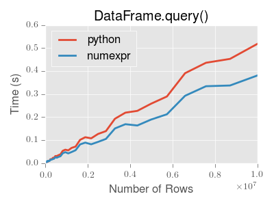
Note
You will only see the performance benefits of using the numexpr engine with DataFrame.query() if your frame has more than approximately 200,000 rows
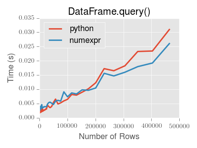
This plot was created using a DataFrame with 3 columns each containing floating point values generated using numpy.random.randn().
Duplicate Data
If you want to identify and remove duplicate rows in a DataFrame, there are two methods that will help: duplicated and drop_duplicates. Each takes as an argument the columns to use to identify duplicated rows.
- duplicated returns a boolean vector whose length is the number of rows, and which indicates whether a row is duplicated.
- drop_duplicates removes duplicate rows.
By default, the first observed row of a duplicate set is considered unique, but each method has a take_last parameter that indicates the last observed row should be taken instead.
In [208]: df2 = DataFrame({'a' : ['one', 'one', 'two', 'three', 'two', 'one', 'six'],
   .....:                  'b' : ['x', 'y', 'y', 'x', 'y', 'x', 'x'],
   .....:                  'c' : np.random.randn(7)})
   .....:

In [209]: df2.duplicated(['a','b'])
Out[209]:
0    False
1    False
2    False
3    False
4     True
5     True
6    False
dtype: bool

In [210]: df2.drop_duplicates(['a','b'])
Out[210]:
       a  b         c
0    one  x  0.932713
1    one  y -0.393510
2    two  y -0.548454
3  three  x  1.130736
6    six  x -1.233298

In [211]: df2.drop_duplicates(['a','b'], take_last=True)
Out[211]:
       a  b         c
1    one  y -0.393510
3  three  x  1.130736
4    two  y -0.447217
5    one  x  1.043921
6    six  x -1.233298
Dictionary-like get() method
Each of Series, DataFrame, and Panel have a get method which can return a default value.
In [212]: s = Series([1,2,3], index=['a','b','c'])

In [213]: s.get('a')               # equivalent to s['a']
Out[213]: 1

In [214]: s.get('x', default=-1)
Out[214]: -1
The select() Method
Another way to extract slices from an object is with the select method of Series, DataFrame, and Panel. This method should be used only when there is no more direct way. select takes a function which operates on labels along axis and returns a boolean. For instance:
In [215]: df.select(lambda x: x == 'A', axis=1)
Out[215]:
                   A
2000-01-01  0.454389
2000-01-02  0.036249
2000-01-03  0.378125
2000-01-04  0.075871
2000-01-05 -0.677097
2000-01-06  1.482845
2000-01-07  0.272681
2000-01-08 -0.459059
The lookup() Method
Sometimes you want to extract a set of values given a sequence of row labels and column labels, and the lookup method allows for this and returns a numpy array. For instance,
In [216]: dflookup = DataFrame(np.random.rand(20,4), columns = ['A','B','C','D'])

In [217]: dflookup.lookup(list(range(0,10,2)), ['B','C','A','B','D'])
Out[217]: array([ 0.012 ,  0.3551,  0.3261,  0.4702,  0.3107])
Index objects
The pandas Index class and its subclasses can be viewed as implementing an ordered multiset. Duplicates are allowed. However, if you try to convert an Index object with duplicate entries into a set, an exception will be raised.
Index also provides the infrastructure necessary for lookups, data alignment, and reindexing. The easiest way to create an Index directly is to pass a list or other sequence to Index:
In [218]: index = Index(['e', 'd', 'a', 'b'])

In [219]: index
Out[219]: Index([u'e', u'd', u'a', u'b'], dtype='object')

In [220]: 'd' in index
Out[220]: True
You can also pass a name to be stored in the index:
In [221]: index = Index(['e', 'd', 'a', 'b'], name='something')

In [222]: index.name
Out[222]: 'something'
The name, if set, will be shown in the console display:
In [223]: index = Index(list(range(5)), name='rows')

In [224]: columns = Index(['A', 'B', 'C'], name='cols')

In [225]: df = DataFrame(np.random.randn(5, 3), index=index, columns=columns)

In [226]: df
Out[226]:
cols         A         B         C
rows
0     0.603791  0.388713  0.544331
1    -0.152978  1.929541  0.202138
2     0.024972  0.117533 -0.184740
3     1.054144 -0.736061 -0.785352
4    -1.362549 -0.063514  0.487562

In [227]: df['A']
Out[227]:
rows
0       0.603791
1      -0.152978
2       0.024972
3       1.054144
4      -1.362549
Name: A, dtype: float64
Setting metadata
New in version 0.13.0.
Indexes are “mostly immutable”, but it is possible to set and change their metadata, like the index name (or, for MultiIndex, levels and labels).
You can use the rename, set_names, set_levels, and set_labels to set these attributes directly. They default to returning a copy; however, you can specify inplace=True to have the data change in place.
See Advanced Indexing for usage of MultiIndexes.
In [228]: ind = Index([1, 2, 3])

In [229]: ind.rename("apple")
Out[229]: Int64Index([1, 2, 3], dtype='int64')

In [230]: ind
Out[230]: Int64Index([1, 2, 3], dtype='int64')

In [231]: ind.set_names(["apple"], inplace=True)

In [232]: ind.name = "bob"

In [233]: ind
Out[233]: Int64Index([1, 2, 3], dtype='int64')
New in version 0.15.0.
set_names, set_levels, and set_labels also take an optional level` argument
In [234]: index = MultiIndex.from_product([range(3), ['one', 'two']], names=['first', 'second'])

In [235]: index
Out[235]:
MultiIndex(levels=[[0, 1, 2], [u'one', u'two']],
           labels=[[0, 0, 1, 1, 2, 2], [0, 1, 0, 1, 0, 1]],
           names=[u'first', u'second'])

In [236]: index.levels[1]
Out[236]: Index([u'one', u'two'], dtype='object')

In [237]: index.set_levels(["a", "b"], level=1)
Out[237]:
MultiIndex(levels=[[0, 1, 2], [u'a', u'b']],
           labels=[[0, 0, 1, 1, 2, 2], [0, 1, 0, 1, 0, 1]],
           names=[u'first', u'second'])
Set operations on Index objects
Warning
In 0.15.0. the set operations + and - were deprecated in order to provide these for numeric type operations on certain index types. + can be replace by .union() or |, and - by .difference().
The two main operations are union (|), intersection (&) These can be directly called as instance methods or used via overloaded operators. Difference is provided via the .difference() method.
In [238]: a = Index(['c', 'b', 'a'])

In [239]: b = Index(['c', 'e', 'd'])

In [240]: a | b
Out[240]: Index([u'a', u'b', u'c', u'd', u'e'], dtype='object')

In [241]: a & b
Out[241]: Index([u'c'], dtype='object')

In [242]: a.difference(b)
Out[242]: Index([u'a', u'b'], dtype='object')
Also available is the sym_diff (^) operation, which returns elements that appear in either idx1 or idx2 but not both. This is equivalent to the Index created by idx1.difference(idx2).union(idx2.difference(idx1)), with duplicates dropped.
In [243]: idx1 = Index([1, 2, 3, 4])

In [244]: idx2 = Index([2, 3, 4, 5])

In [245]: idx1.sym_diff(idx2)
Out[245]: Int64Index([1, 5], dtype='int64')

In [246]: idx1 ^ idx2
Out[246]: Int64Index([1, 5], dtype='int64')
Set / Reset Index
Occasionally you will load or create a data set into a DataFrame and want to add an index after you’ve already done so. There are a couple of different ways.
Set an index
DataFrame has a set_index method which takes a column name (for a regular Index) or a list of column names (for a MultiIndex), to create a new, indexed DataFrame:
In [247]: data
Out[247]:
     a    b  c  d
0  bar  one  z  1
1  bar  two  y  2
2  foo  one  x  3
3  foo  two  w  4

In [248]: indexed1 = data.set_index('c')

In [249]: indexed1
Out[249]:
     a    b  d
c
z  bar  one  1
y  bar  two  2
x  foo  one  3
w  foo  two  4

In [250]: indexed2 = data.set_index(['a', 'b'])

In [251]: indexed2
Out[251]:
         c  d
a   b
bar one  z  1
    two  y  2
foo one  x  3
    two  w  4
The append keyword option allow you to keep the existing index and append the given columns to a MultiIndex:
In [252]: frame = data.set_index('c', drop=False)

In [253]: frame = frame.set_index(['a', 'b'], append=True)

In [254]: frame
Out[254]:
           c  d
c a   b
z bar one  z  1
y bar two  y  2
x foo one  x  3
w foo two  w  4
Other options in set_index allow you not drop the index columns or to add the index in-place (without creating a new object):
In [255]: data.set_index('c', drop=False)
Out[255]:
     a    b  c  d
c
z  bar  one  z  1
y  bar  two  y  2
x  foo  one  x  3
w  foo  two  w  4

In [256]: data.set_index(['a', 'b'], inplace=True)

In [257]: data
Out[257]:
         c  d
a   b
bar one  z  1
    two  y  2
foo one  x  3
    two  w  4
Reset the index
As a convenience, there is a new function on DataFrame called reset_index which transfers the index values into the DataFrame’s columns and sets a simple integer index. This is the inverse operation to set_index
In [258]: data
Out[258]:
         c  d
a   b
bar one  z  1
    two  y  2
foo one  x  3
    two  w  4

In [259]: data.reset_index()
Out[259]:
     a    b  c  d
0  bar  one  z  1
1  bar  two  y  2
2  foo  one  x  3
3  foo  two  w  4
The output is more similar to a SQL table or a record array. The names for the columns derived from the index are the ones stored in the names attribute.
You can use the level keyword to remove only a portion of the index:
In [260]: frame
Out[260]:
           c  d
c a   b
z bar one  z  1
y bar two  y  2
x foo one  x  3
w foo two  w  4

In [261]: frame.reset_index(level=1)
Out[261]:
         a  c  d
c b
z one  bar  z  1
y two  bar  y  2
x one  foo  x  3
w two  foo  w  4
reset_index takes an optional parameter drop which if true simply discards the index, instead of putting index values in the DataFrame’s columns.
Note
The reset_index method used to be called delevel which is now deprecated.
Adding an ad hoc index
If you create an index yourself, you can just assign it to the index field:
data.index = index
Returning a view versus a copy
When setting values in a pandas object, care must be taken to avoid what is called chained indexing. Here is an example.
In [262]: dfmi = DataFrame([list('abcd'),
   .....:                   list('efgh'),
   .....:                   list('ijkl'),
   .....:                   list('mnop')],
   .....:                  columns=MultiIndex.from_product([['one','two'],
   .....:                                                   ['first','second']]))
   .....:

In [263]: dfmi
Out[263]:
    one          two
  first second first second
0     a      b     c      d
1     e      f     g      h
2     i      j     k      l
3     m      n     o      p
Compare these two access methods:
In [264]: dfmi['one']['second']
Out[264]:
0    b
1    f
2    j
3    n
Name: second, dtype: object
In [265]: dfmi.loc[:,('one','second')]
Out[265]:
0    b
1    f
2    j
3    n
Name: (one, second), dtype: object
These both yield the same results, so which should you use? It is instructive to understand the order of operations on these and why method 2 (.loc) is much preferred over method 1 (chained [])
dfmi['one'] selects the first level of the columns and returns a data frame that is singly-indexed. Then another python operation dfmi_with_one['second'] selects the series indexed by 'second' happens. This is indicated by the variable dfmi_with_one because pandas sees these operations as separate events. e.g. separate calls to __getitem__, so it has to treat them as linear operations, they happen one after another.
Contrast this to df.loc[:,('one','second')] which passes a nested tuple of (slice(None),('one','second')) to a single call to __getitem__. This allows pandas to deal with this as a single entity. Furthermore this order of operations can be significantly faster, and allows one to index both axes if so desired.
Why does the assignment when using chained indexing fail!
So, why does this show the SettingWithCopy warning / and possibly not work when you do chained indexing and assignment:
dfmi['one']['second'] = value
Since the chained indexing is 2 calls, it is possible that either call may return a copy of the data because of the way it is sliced. Thus when setting, you are actually setting a copy, and not the original frame data. It is impossible for pandas to figure this out because their are 2 separate python operations that are not connected.
The SettingWithCopy warning is a ‘heuristic’ to detect this (meaning it tends to catch most cases but is simply a lightweight check). Figuring this out for real is way complicated.
The .loc operation is a single python operation, and thus can select a slice (which still may be a copy), but allows pandas to assign that slice back into the frame after it is modified, thus setting the values as you would think.
The reason for having the SettingWithCopy warning is this. Sometimes when you slice an array you will simply get a view back, which means you can set it no problem. However, even a single dtyped array can generate a copy if it is sliced in a particular way. A multi-dtyped DataFrame (meaning it has say float and object data), will almost always yield a copy. Whether a view is created is dependent on the memory layout of the array.
Evaluation order matters
Furthermore, in chained expressions, the order may determine whether a copy is returned or not. If an expression will set values on a copy of a slice, then a SettingWithCopy exception will be raised (this raise/warn behavior is new starting in 0.13.0)
You can control the action of a chained assignment via the option mode.chained_assignment, which can take the values ['raise','warn',None], where showing a warning is the default.
In [266]: dfb = DataFrame({'a' : ['one', 'one', 'two',
   .....:                         'three', 'two', 'one', 'six'],
   .....:                  'c' : np.arange(7)})
   .....:

# This will show the SettingWithCopyWarning
# but the frame values will be set
In [267]: dfb['c'][dfb.a.str.startswith('o')] = 42
This however is operating on a copy and will not work.
>>> pd.set_option('mode.chained_assignment','warn')
>>> dfb[dfb.a.str.startswith('o')]['c'] = 42
Traceback (most recent call last)
     ...
SettingWithCopyWarning:
     A value is trying to be set on a copy of a slice from a DataFrame.
     Try using .loc[row_index,col_indexer] = value instead
A chained assignment can also crop up in setting in a mixed dtype frame.
Note
These setting rules apply to all of .loc/.iloc/.ix
This is the correct access method
In [268]: dfc = DataFrame({'A':['aaa','bbb','ccc'],'B':[1,2,3]})

In [269]: dfc.loc[0,'A'] = 11

In [270]: dfc
Out[270]:
     A  B
0   11  1
1  bbb  2
2  ccc  3
This can work at times, but is not guaranteed, and so should be avoided
In [271]: dfc = dfc.copy()

In [272]: dfc['A'][0] = 111

In [273]: dfc
Out[273]:
     A  B
0  111  1
1  bbb  2
2  ccc  3
This will not work at all, and so should be avoided
>>> pd.set_option('mode.chained_assignment','raise')
>>> dfc.loc[0]['A'] = 1111
Traceback (most recent call last)
     ...
SettingWithCopyException:
     A value is trying to be set on a copy of a slice from a DataFrame.
     Try using .loc[row_index,col_indexer] = value instead
Warning
The chained assignment warnings / exceptions are aiming to inform the user of a possibly invalid assignment. There may be false positives; situations where a chained assignment is inadvertantly reported.