Computational tools
Statistical Functions
Percent Change
Series, DataFrame, and Panel all have a method pct_change to compute the percent change over a given number of periods (using fill_method to fill NA/null values before computing the percent change).
In [1]: ser = pd.Series(np.random.randn(8))

In [2]: ser.pct_change()
Out[2]:
0         NaN
1   -1.602976
2    4.334938
3   -0.247456
4   -2.067345
5   -1.142903
6   -1.688214
7   -9.759729
dtype: float64
In [3]: df = pd.DataFrame(np.random.randn(10, 4))

In [4]: df.pct_change(periods=3)
Out[4]:
          0         1         2         3
0       NaN       NaN       NaN       NaN
1       NaN       NaN       NaN       NaN
2       NaN       NaN       NaN       NaN
3 -0.218320 -1.054001  1.987147 -0.510183
4 -0.439121 -1.816454  0.649715 -4.822809
5 -0.127833 -3.042065 -5.866604 -1.776977
6 -2.596833 -1.959538 -2.111697 -3.798900
7 -0.117826 -2.169058  0.036094 -0.067696
8  2.492606 -1.357320 -1.205802 -1.558697
9 -1.012977  2.324558 -1.003744 -0.371806
Covariance
The Series object has a method cov to compute covariance between series (excluding NA/null values).
In [5]: s1 = pd.Series(np.random.randn(1000))

In [6]: s2 = pd.Series(np.random.randn(1000))

In [7]: s1.cov(s2)
Out[7]: 0.00068010881743110698
Analogously, DataFrame has a method cov to compute pairwise covariances among the series in the DataFrame, also excluding NA/null values.
Note
Assuming the missing data are missing at random this results in an estimate for the covariance matrix which is unbiased. However, for many applications this estimate may not be acceptable because the estimated covariance matrix is not guaranteed to be positive semi-definite. This could lead to estimated correlations having absolute values which are greater than one, and/or a non-invertible covariance matrix. See Estimation of covariance matrices for more details.
In [8]: frame = pd.DataFrame(np.random.randn(1000, 5), columns=['a', 'b', 'c', 'd', 'e'])

In [9]: frame.cov()
Out[9]:
          a         b         c         d         e
a  1.000882 -0.003177 -0.002698 -0.006889  0.031912
b -0.003177  1.024721  0.000191  0.009212  0.000857
c -0.002698  0.000191  0.950735 -0.031743 -0.005087
d -0.006889  0.009212 -0.031743  1.002983 -0.047952
e  0.031912  0.000857 -0.005087 -0.047952  1.042487
DataFrame.cov also supports an optional min_periods keyword that specifies the required minimum number of observations for each column pair in order to have a valid result.
In [10]: frame = pd.DataFrame(np.random.randn(20, 3), columns=['a', 'b', 'c'])

In [11]: frame.ix[:5, 'a'] = np.nan

In [12]: frame.ix[5:10, 'b'] = np.nan

In [13]: frame.cov()
Out[13]:
          a         b         c
a  1.210090 -0.430629  0.018002
b -0.430629  1.240960  0.347188
c  0.018002  0.347188  1.301149

In [14]: frame.cov(min_periods=12)
Out[14]:
          a         b         c
a  1.210090       NaN  0.018002
b       NaN  1.240960  0.347188
c  0.018002  0.347188  1.301149
Correlation
Several methods for computing correlations are provided:
| Method name | Description |
|---|---|
| pearson (default) | Standard correlation coefficient |
| kendall | Kendall Tau correlation coefficient |
| spearman | Spearman rank correlation coefficient |
All of these are currently computed using pairwise complete observations.
Note
Please see the caveats associated with this method of calculating correlation matrices in the covariance section.
In [15]: frame = pd.DataFrame(np.random.randn(1000, 5), columns=['a', 'b', 'c', 'd', 'e'])

In [16]: frame.ix[::2] = np.nan

# Series with Series
In [17]: frame['a'].corr(frame['b'])
Out[17]: 0.013479040400098789

In [18]: frame['a'].corr(frame['b'], method='spearman')
Out[18]: -0.0072898851595406388

# Pairwise correlation of DataFrame columns
In [19]: frame.corr()
Out[19]:
          a         b         c         d         e
a  1.000000  0.013479 -0.049269 -0.042239 -0.028525
b  0.013479  1.000000 -0.020433 -0.011139  0.005654
c -0.049269 -0.020433  1.000000  0.018587 -0.054269
d -0.042239 -0.011139  0.018587  1.000000 -0.017060
e -0.028525  0.005654 -0.054269 -0.017060  1.000000
Note that non-numeric columns will be automatically excluded from the correlation calculation.
Like cov, corr also supports the optional min_periods keyword:
In [20]: frame = pd.DataFrame(np.random.randn(20, 3), columns=['a', 'b', 'c'])

In [21]: frame.ix[:5, 'a'] = np.nan

In [22]: frame.ix[5:10, 'b'] = np.nan

In [23]: frame.corr()
Out[23]:
          a         b         c
a  1.000000 -0.076520  0.160092
b -0.076520  1.000000  0.135967
c  0.160092  0.135967  1.000000

In [24]: frame.corr(min_periods=12)
Out[24]:
          a         b         c
a  1.000000       NaN  0.160092
b       NaN  1.000000  0.135967
c  0.160092  0.135967  1.000000
A related method corrwith is implemented on DataFrame to compute the correlation between like-labeled Series contained in different DataFrame objects.
In [25]: index = ['a', 'b', 'c', 'd', 'e']

In [26]: columns = ['one', 'two', 'three', 'four']

In [27]: df1 = pd.DataFrame(np.random.randn(5, 4), index=index, columns=columns)

In [28]: df2 = pd.DataFrame(np.random.randn(4, 4), index=index[:4], columns=columns)

In [29]: df1.corrwith(df2)
Out[29]:
one     -0.125501
two     -0.493244
three    0.344056
four     0.004183
dtype: float64

In [30]: df2.corrwith(df1, axis=1)
Out[30]:
a   -0.675817
b    0.458296
c    0.190809
d   -0.186275
e         NaN
dtype: float64
Data ranking
The rank method produces a data ranking with ties being assigned the mean of the ranks (by default) for the group:
In [31]: s = pd.Series(np.random.np.random.randn(5), index=list('abcde'))

In [32]: s['d'] = s['b'] # so there's a tie

In [33]: s.rank()
Out[33]:
a    5.0
b    2.5
c    1.0
d    2.5
e    4.0
dtype: float64
rank is also a DataFrame method and can rank either the rows (axis=0) or the columns (axis=1). NaN values are excluded from the ranking.
In [34]: df = pd.DataFrame(np.random.np.random.randn(10, 6))

In [35]: df[4] = df[2][:5] # some ties

In [36]: df
Out[36]:
          0         1         2         3         4         5
0 -0.904948 -1.163537 -1.457187  0.135463 -1.457187  0.294650
1 -0.976288 -0.244652 -0.748406 -0.999601 -0.748406 -0.800809
2  0.401965  1.460840  1.256057  1.308127  1.256057  0.876004
3  0.205954  0.369552 -0.669304  0.038378 -0.669304  1.140296
4 -0.477586 -0.730705 -1.129149 -0.601463 -1.129149 -0.211196
5 -1.092970 -0.689246  0.908114  0.204848       NaN  0.463347
6  0.376892  0.959292  0.095572 -0.593740       NaN -0.069180
7 -1.002601  1.957794 -0.120708  0.094214       NaN -1.467422
8 -0.547231  0.664402 -0.519424 -0.073254       NaN -1.263544
9 -0.250277 -0.237428 -1.056443  0.419477       NaN  1.375064

In [37]: df.rank(1)
Out[37]:
     0    1    2    3    4    5
0  4.0  3.0  1.5  5.0  1.5  6.0
1  2.0  6.0  4.5  1.0  4.5  3.0
2  1.0  6.0  3.5  5.0  3.5  2.0
3  4.0  5.0  1.5  3.0  1.5  6.0
4  5.0  3.0  1.5  4.0  1.5  6.0
5  1.0  2.0  5.0  3.0  NaN  4.0
6  4.0  5.0  3.0  1.0  NaN  2.0
7  2.0  5.0  3.0  4.0  NaN  1.0
8  2.0  5.0  3.0  4.0  NaN  1.0
9  2.0  3.0  1.0  4.0  NaN  5.0
rank optionally takes a parameter ascending which by default is true; when false, data is reverse-ranked, with larger values assigned a smaller rank.
rank supports different tie-breaking methods, specified with the method parameter:
- average : average rank of tied group
- min : lowest rank in the group
- max : highest rank in the group
- first : ranks assigned in the order they appear in the array
Window Functions
Warning
Prior to version 0.18.0, pd.rolling_*, pd.expanding_*, and pd.ewm* were module level functions and are now deprecated. These are replaced by using the Rolling, Expanding and EWM. objects and a corresponding method call.
The deprecation warning will show the new syntax, see an example here You can view the previous documentation here
For working with data, a number of windows functions are provided for computing common window or rolling statistics. Among these are count, sum, mean, median, correlation, variance, covariance, standard deviation, skewness, and kurtosis.
Note
The API for window statistics is quite similar to the way one works with GroupBy objects, see the documentation here
We work with rolling, expanding and exponentially weighted data through the corresponding objects, Rolling, Expanding and EWM.
In [38]: s = pd.Series(np.random.randn(1000), index=pd.date_range('1/1/2000', periods=1000))

In [39]: s = s.cumsum()

In [40]: s
Out[40]:
2000-01-01    -0.268824
2000-01-02    -1.771855
2000-01-03    -0.818003
2000-01-04    -0.659244
2000-01-05    -1.942133
2000-01-06    -1.869391
2000-01-07     0.563674
                ...
2002-09-20   -68.233054
2002-09-21   -66.765687
2002-09-22   -67.457323
2002-09-23   -69.253182
2002-09-24   -70.296818
2002-09-25   -70.844674
2002-09-26   -72.475016
Freq: D, dtype: float64
These are created from methods on Series and DataFrame.
In [41]: r = s.rolling(window=60)

In [42]: r
Out[42]: Rolling [window=60,center=False,axis=0]
These object provide tab-completion of the avaible methods and properties.
In [14]: r.
r.agg         r.apply       r.count       r.exclusions  r.max         r.median      r.name        r.skew        r.sum
r.aggregate   r.corr        r.cov         r.kurt        r.mean        r.min         r.quantile    r.std         r.var
Generally these methods all have the same interface. They all accept the following arguments:
- window: size of moving window
- min_periods: threshold of non-null data points to require (otherwise result is NA)
- center: boolean, whether to set the labels at the center (default is False)
Warning
The freq and how arguments were in the API prior to 0.18.0 changes. These are deprecated in the new API. You can simply resample the input prior to creating a window function.
For example, instead of s.rolling(window=5,freq='D').max() to get the max value on a rolling 5 Day window, one could use s.resample('D').max().rolling(window=5).max(), which first resamples the data to daily data, then provides a rolling 5 day window.
We can then call methods on these rolling objects. These return like-indexed objects:
In [43]: r.mean()
Out[43]:
2000-01-01          NaN
2000-01-02          NaN
2000-01-03          NaN
2000-01-04          NaN
2000-01-05          NaN
2000-01-06          NaN
2000-01-07          NaN
                ...
2002-09-20   -62.694135
2002-09-21   -62.812190
2002-09-22   -62.914971
2002-09-23   -63.061867
2002-09-24   -63.213876
2002-09-25   -63.375074
2002-09-26   -63.539734
Freq: D, dtype: float64
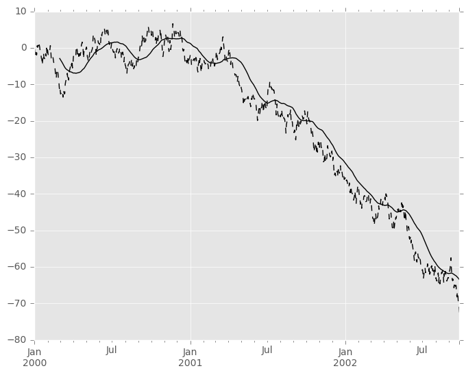
In [44]: s.plot(style='k--')
Out[44]: <matplotlib.axes._subplots.AxesSubplot at 0x11ce37110>

In [45]: r.mean().plot(style='k')
Out[45]: <matplotlib.axes._subplots.AxesSubplot at 0x11ce37110>
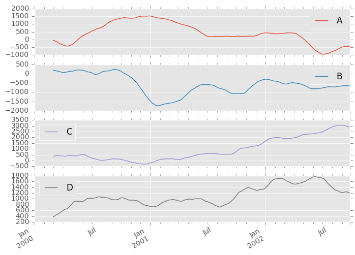
They can also be applied to DataFrame objects. This is really just syntactic sugar for applying the moving window operator to all of the DataFrame’s columns:
In [46]: df = pd.DataFrame(np.random.randn(1000, 4),
   ....:                   index=pd.date_range('1/1/2000', periods=1000),
   ....:                   columns=['A', 'B', 'C', 'D'])
   ....:

In [47]: df = df.cumsum()

In [48]: df.rolling(window=60).sum().plot(subplots=True)
Out[48]:
array([<matplotlib.axes._subplots.AxesSubplot object at 0x11cdc2890>,
       <matplotlib.axes._subplots.AxesSubplot object at 0x120dfef50>,
       <matplotlib.axes._subplots.AxesSubplot object at 0x120cd4110>,
       <matplotlib.axes._subplots.AxesSubplot object at 0x1127f6e90>], dtype=object)
Method Summary
We provide a number of the common statistical functions:
| Method | Description |
|---|---|
| count() | Number of non-null observations |
| sum() | Sum of values |
| mean() | Mean of values |
| median() | Arithmetic median of values |
| min() | Minimum |
| max() | Maximum |
| std() | Bessel-corrected sample standard deviation |
| var() | Unbiased variance |
| skew() | Sample skewness (3rd moment) |
| kurt() | Sample kurtosis (4th moment) |
| quantile() | Sample quantile (value at %) |
| apply() | Generic apply |
| cov() | Unbiased covariance (binary) |
| corr() | Correlation (binary) |
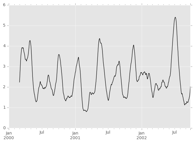
The apply() function takes an extra func argument and performs generic rolling computations. The func argument should be a single function that produces a single value from an ndarray input. Suppose we wanted to compute the mean absolute deviation on a rolling basis:
In [49]: mad = lambda x: np.fabs(x - x.mean()).mean()

In [50]: s.rolling(window=60).apply(mad).plot(style='k')
Out[50]: <matplotlib.axes._subplots.AxesSubplot at 0x112f25950>
Rolling Windows
Passing win_type to .rolling generates a generic rolling window computation, that is weighted according the win_type. The following methods are available:
| Method | Description |
|---|---|
| sum() | Sum of values |
| mean() | Mean of values |
The weights used in the window are specified by the win_type keyword. The list of recognized types are:
- boxcar
- triang
- blackman
- hamming
- bartlett
- parzen
- bohman
- blackmanharris
- nuttall
- barthann
- kaiser (needs beta)
- gaussian (needs std)
- general_gaussian (needs power, width)
- slepian (needs width).
In [51]: ser = pd.Series(np.random.randn(10), index=pd.date_range('1/1/2000', periods=10))

In [52]: ser.rolling(window=5, win_type='triang').mean()
Out[52]:
2000-01-01         NaN
2000-01-02         NaN
2000-01-03         NaN
2000-01-04         NaN
2000-01-05   -1.037870
2000-01-06   -0.767705
2000-01-07   -0.383197
2000-01-08   -0.395513
2000-01-09   -0.558440
2000-01-10   -0.672416
Freq: D, dtype: float64
Note that the boxcar window is equivalent to mean().
In [53]: ser.rolling(window=5, win_type='boxcar').mean()
Out[53]:
2000-01-01         NaN
2000-01-02         NaN
2000-01-03         NaN
2000-01-04         NaN
2000-01-05   -0.841164
2000-01-06   -0.779948
2000-01-07   -0.565487
2000-01-08   -0.502815
2000-01-09   -0.553755
2000-01-10   -0.472211
Freq: D, dtype: float64

In [54]: ser.rolling(window=5).mean()
Out[54]:
2000-01-01         NaN
2000-01-02         NaN
2000-01-03         NaN
2000-01-04         NaN
2000-01-05   -0.841164
2000-01-06   -0.779948
2000-01-07   -0.565487
2000-01-08   -0.502815
2000-01-09   -0.553755
2000-01-10   -0.472211
Freq: D, dtype: float64
For some windowing functions, additional parameters must be specified:
In [55]: ser.rolling(window=5, win_type='gaussian').mean(std=0.1)
Out[55]:
2000-01-01         NaN
2000-01-02         NaN
2000-01-03         NaN
2000-01-04         NaN
2000-01-05   -1.309989
2000-01-06   -1.153000
2000-01-07    0.606382
2000-01-08   -0.681101
2000-01-09   -0.289724
2000-01-10   -0.996632
Freq: D, dtype: float64
Note
For .sum() with a win_type, there is no normalization done to the weights for the window. Passing custom weights of [1, 1, 1] will yield a different result than passing weights of [2, 2, 2], for example. When passing a win_type instead of explicitly specifying the weights, the weights are already normalized so that the largest weight is 1.
In contrast, the nature of the .mean() calculation is such that the weights are normalized with respect to each other. Weights of [1, 1, 1] and [2, 2, 2] yield the same result.
Centering Windows
By default the labels are set to the right edge of the window, but a center keyword is available so the labels can be set at the center.
In [56]: ser.rolling(window=5).mean()
Out[56]:
2000-01-01         NaN
2000-01-02         NaN
2000-01-03         NaN
2000-01-04         NaN
2000-01-05   -0.841164
2000-01-06   -0.779948
2000-01-07   -0.565487
2000-01-08   -0.502815
2000-01-09   -0.553755
2000-01-10   -0.472211
Freq: D, dtype: float64

In [57]: ser.rolling(window=5, center=True).mean()
Out[57]:
2000-01-01         NaN
2000-01-02         NaN
2000-01-03   -0.841164
2000-01-04   -0.779948
2000-01-05   -0.565487
2000-01-06   -0.502815
2000-01-07   -0.553755
2000-01-08   -0.472211
2000-01-09         NaN
2000-01-10         NaN
Freq: D, dtype: float64
Binary Window Functions
cov() and corr() can compute moving window statistics about two Series or any combination of DataFrame/Series or DataFrame/DataFrame. Here is the behavior in each case:
- two Series: compute the statistic for the pairing.
- DataFrame/Series: compute the statistics for each column of the DataFrame with the passed Series, thus returning a DataFrame.
- DataFrame/DataFrame: by default compute the statistic for matching column names, returning a DataFrame. If the keyword argument pairwise=True is passed then computes the statistic for each pair of columns, returning a Panel whose items are the dates in question (see the next section).
For example:
In [58]: df2 = df[:20]

In [59]: df2.rolling(window=5).corr(df2['B'])
Out[59]:
                   A    B         C         D
2000-01-01       NaN  NaN       NaN       NaN
2000-01-02       NaN  NaN       NaN       NaN
2000-01-03       NaN  NaN       NaN       NaN
2000-01-04       NaN  NaN       NaN       NaN
2000-01-05 -0.262853  1.0  0.334449  0.193380
2000-01-06 -0.083745  1.0 -0.521587 -0.556126
2000-01-07 -0.292940  1.0 -0.658532 -0.458128
...              ...  ...       ...       ...
2000-01-14  0.519499  1.0 -0.687277  0.192822
2000-01-15  0.048982  1.0  0.167669 -0.061463
2000-01-16  0.217190  1.0  0.167564 -0.326034
2000-01-17  0.641180  1.0 -0.164780 -0.111487
2000-01-18  0.130422  1.0  0.322833  0.632383
2000-01-19  0.317278  1.0  0.384528  0.813656
2000-01-20  0.293598  1.0  0.159538  0.742381

[20 rows x 4 columns]
Computing rolling pairwise covariances and correlations
In financial data analysis and other fields it’s common to compute covariance and correlation matrices for a collection of time series. Often one is also interested in moving-window covariance and correlation matrices. This can be done by passing the pairwise keyword argument, which in the case of DataFrame inputs will yield a Panel whose items are the dates in question. In the case of a single DataFrame argument the pairwise argument can even be omitted:
Note
Missing values are ignored and each entry is computed using the pairwise complete observations. Please see the covariance section for caveats associated with this method of calculating covariance and correlation matrices.
In [60]: covs = df[['B','C','D']].rolling(window=50).cov(df[['A','B','C']], pairwise=True)

In [61]: covs[df.index[-50]]
Out[61]:
          A         B          C
B  2.667506  1.671711   1.938634
C  8.513843  1.938634  10.556436
D -7.714737 -1.434529  -7.082653
In [62]: correls = df.rolling(window=50).corr()

In [63]: correls[df.index[-50]]
Out[63]:
          A         B         C         D
A  1.000000  0.604221  0.767429 -0.776170
B  0.604221  1.000000  0.461484 -0.381148
C  0.767429  0.461484  1.000000 -0.748863
D -0.776170 -0.381148 -0.748863  1.000000
You can efficiently retrieve the time series of correlations between two columns using .loc indexing:
In [64]: correls.loc[:, 'A', 'C'].plot()
Out[64]: <matplotlib.axes._subplots.AxesSubplot at 0x11ea521d0>
Aggregation
Once the Rolling, Expanding or EWM objects have been created, several methods are available to perform multiple computations on the data. This is very similar to a .groupby(...).agg seen here.
In [65]: dfa = pd.DataFrame(np.random.randn(1000, 3),
   ....:                    index=pd.date_range('1/1/2000', periods=1000),
   ....:                    columns=['A', 'B', 'C'])
   ....:

In [66]: r = dfa.rolling(window=60,min_periods=1)

In [67]: r
Out[67]: Rolling [window=60,min_periods=1,center=False,axis=0]
We can aggregate by passing a function to the entire DataFrame, or select a Series (or multiple Series) via standard getitem.
In [68]: r.aggregate(np.sum)
Out[68]:
                   A          B         C
2000-01-01  0.314226  -0.001675  0.071823
2000-01-02  1.206791   0.678918 -0.267817
2000-01-03  1.421701   0.600508 -0.445482
2000-01-04  1.912539  -0.759594  1.146974
2000-01-05  2.919639  -0.061759 -0.743617
2000-01-06  2.665637   1.298392 -0.803529
2000-01-07  2.513985   1.923089 -1.928308
...              ...        ...       ...
2002-09-20  1.447669 -12.360302  2.734381
2002-09-21  1.871783 -13.896542  3.086102
2002-09-22  2.540658 -12.594402  3.162542
2002-09-23  2.974674 -12.727703  3.861005
2002-09-24  1.391366 -13.584590  3.790683
2002-09-25  2.027313 -15.083214  3.377896
2002-09-26  1.290363 -13.569459  3.809884

[1000 rows x 3 columns]

In [69]: r['A'].aggregate(np.sum)
Out[69]:
2000-01-01    0.314226
2000-01-02    1.206791
2000-01-03    1.421701
2000-01-04    1.912539
2000-01-05    2.919639
2000-01-06    2.665637
2000-01-07    2.513985
                ...
2002-09-20    1.447669
2002-09-21    1.871783
2002-09-22    2.540658
2002-09-23    2.974674
2002-09-24    1.391366
2002-09-25    2.027313
2002-09-26    1.290363
Freq: D, Name: A, dtype: float64

In [70]: r[['A','B']].aggregate(np.sum)
Out[70]:
                   A          B
2000-01-01  0.314226  -0.001675
2000-01-02  1.206791   0.678918
2000-01-03  1.421701   0.600508
2000-01-04  1.912539  -0.759594
2000-01-05  2.919639  -0.061759
2000-01-06  2.665637   1.298392
2000-01-07  2.513985   1.923089
...              ...        ...
2002-09-20  1.447669 -12.360302
2002-09-21  1.871783 -13.896542
2002-09-22  2.540658 -12.594402
2002-09-23  2.974674 -12.727703
2002-09-24  1.391366 -13.584590
2002-09-25  2.027313 -15.083214
2002-09-26  1.290363 -13.569459

[1000 rows x 2 columns]
As you can see, the result of the aggregation will have the selected columns, or all columns if none are selected.
Applying multiple functions at once
With windowed Series you can also pass a list or dict of functions to do aggregation with, outputting a DataFrame:
In [71]: r['A'].agg([np.sum, np.mean, np.std])
Out[71]:
                 sum      mean       std
2000-01-01  0.314226  0.314226       NaN
2000-01-02  1.206791  0.603396  0.408948
2000-01-03  1.421701  0.473900  0.365959
2000-01-04  1.912539  0.478135  0.298925
2000-01-05  2.919639  0.583928  0.350682
2000-01-06  2.665637  0.444273  0.464115
2000-01-07  2.513985  0.359141  0.479828
...              ...       ...       ...
2002-09-20  1.447669  0.024128  1.034827
2002-09-21  1.871783  0.031196  1.031417
2002-09-22  2.540658  0.042344  1.026341
2002-09-23  2.974674  0.049578  1.030021
2002-09-24  1.391366  0.023189  1.024793
2002-09-25  2.027313  0.033789  1.022099
2002-09-26  1.290363  0.021506  1.024751

[1000 rows x 3 columns]
If a dict is passed, the keys will be used to name the columns. Otherwise the function’s name (stored in the function object) will be used.
In [72]: r['A'].agg({'result1' : np.sum,
   ....:             'result2' : np.mean})
   ....:
Out[72]:
             result2   result1
2000-01-01  0.314226  0.314226
2000-01-02  0.603396  1.206791
2000-01-03  0.473900  1.421701
2000-01-04  0.478135  1.912539
2000-01-05  0.583928  2.919639
2000-01-06  0.444273  2.665637
2000-01-07  0.359141  2.513985
...              ...       ...
2002-09-20  0.024128  1.447669
2002-09-21  0.031196  1.871783
2002-09-22  0.042344  2.540658
2002-09-23  0.049578  2.974674
2002-09-24  0.023189  1.391366
2002-09-25  0.033789  2.027313
2002-09-26  0.021506  1.290363

[1000 rows x 2 columns]
On a widowed DataFrame, you can pass a list of functions to apply to each column, which produces an aggregated result with a hierarchical index:
In [73]: r.agg([np.sum, np.mean])
Out[73]:
                   A                    B                   C
                 sum      mean        sum      mean       sum      mean
2000-01-01  0.314226  0.314226  -0.001675 -0.001675  0.071823  0.071823
2000-01-02  1.206791  0.603396   0.678918  0.339459 -0.267817 -0.133908
2000-01-03  1.421701  0.473900   0.600508  0.200169 -0.445482 -0.148494
2000-01-04  1.912539  0.478135  -0.759594 -0.189899  1.146974  0.286744
2000-01-05  2.919639  0.583928  -0.061759 -0.012352 -0.743617 -0.148723
2000-01-06  2.665637  0.444273   1.298392  0.216399 -0.803529 -0.133921
2000-01-07  2.513985  0.359141   1.923089  0.274727 -1.928308 -0.275473
...              ...       ...        ...       ...       ...       ...
2002-09-20  1.447669  0.024128 -12.360302 -0.206005  2.734381  0.045573
2002-09-21  1.871783  0.031196 -13.896542 -0.231609  3.086102  0.051435
2002-09-22  2.540658  0.042344 -12.594402 -0.209907  3.162542  0.052709
2002-09-23  2.974674  0.049578 -12.727703 -0.212128  3.861005  0.064350
2002-09-24  1.391366  0.023189 -13.584590 -0.226410  3.790683  0.063178
2002-09-25  2.027313  0.033789 -15.083214 -0.251387  3.377896  0.056298
2002-09-26  1.290363  0.021506 -13.569459 -0.226158  3.809884  0.063498

[1000 rows x 6 columns]
Passing a dict of functions has different behavior by default, see the next section.
Applying different functions to DataFrame columns
By passing a dict to aggregate you can apply a different aggregation to the columns of a DataFrame:
In [74]: r.agg({'A' : np.sum,
   ....:        'B' : lambda x: np.std(x, ddof=1)})
   ....:
Out[74]:
                   A         B
2000-01-01  0.314226       NaN
2000-01-02  1.206791  0.482437
2000-01-03  1.421701  0.417825
2000-01-04  1.912539  0.851468
2000-01-05  2.919639  0.837474
2000-01-06  2.665637  0.935441
2000-01-07  2.513985  0.867770
...              ...       ...
2002-09-20  1.447669  1.084259
2002-09-21  1.871783  1.088368
2002-09-22  2.540658  1.084707
2002-09-23  2.974674  1.084936
2002-09-24  1.391366  1.079268
2002-09-25  2.027313  1.091334
2002-09-26  1.290363  1.060255

[1000 rows x 2 columns]
The function names can also be strings. In order for a string to be valid it must be implemented on the windowed object
In [75]: r.agg({'A' : 'sum', 'B' : 'std'})
Out[75]:
                   A         B
2000-01-01  0.314226       NaN
2000-01-02  1.206791  0.482437
2000-01-03  1.421701  0.417825
2000-01-04  1.912539  0.851468
2000-01-05  2.919639  0.837474
2000-01-06  2.665637  0.935441
2000-01-07  2.513985  0.867770
...              ...       ...
2002-09-20  1.447669  1.084259
2002-09-21  1.871783  1.088368
2002-09-22  2.540658  1.084707
2002-09-23  2.974674  1.084936
2002-09-24  1.391366  1.079268
2002-09-25  2.027313  1.091334
2002-09-26  1.290363  1.060255

[1000 rows x 2 columns]
Furthermore you can pass a nested dict to indicate different aggregations on different columns.
In [76]: r.agg({'A' : ['sum','std'], 'B' : ['mean','std'] })
Out[76]:
                   A                   B
                 sum       std      mean       std
2000-01-01  0.314226       NaN -0.001675       NaN
2000-01-02  1.206791  0.408948  0.339459  0.482437
2000-01-03  1.421701  0.365959  0.200169  0.417825
2000-01-04  1.912539  0.298925 -0.189899  0.851468
2000-01-05  2.919639  0.350682 -0.012352  0.837474
2000-01-06  2.665637  0.464115  0.216399  0.935441
2000-01-07  2.513985  0.479828  0.274727  0.867770
...              ...       ...       ...       ...
2002-09-20  1.447669  1.034827 -0.206005  1.084259
2002-09-21  1.871783  1.031417 -0.231609  1.088368
2002-09-22  2.540658  1.026341 -0.209907  1.084707
2002-09-23  2.974674  1.030021 -0.212128  1.084936
2002-09-24  1.391366  1.024793 -0.226410  1.079268
2002-09-25  2.027313  1.022099 -0.251387  1.091334
2002-09-26  1.290363  1.024751 -0.226158  1.060255

[1000 rows x 4 columns]
Expanding Windows
A common alternative to rolling statistics is to use an expanding window, which yields the value of the statistic with all the data available up to that point in time.
These follow a similar interface to .rolling, with the .expanding method returning an Expanding object.
As these calculations are a special case of rolling statistics, they are implemented in pandas such that the following two calls are equivalent:
In [77]: df.rolling(window=len(df), min_periods=1).mean()[:5]
Out[77]:
                   A         B         C         D
2000-01-01 -1.388345  3.317290  0.344542 -0.036968
2000-01-02 -1.123132  3.622300  1.675867  0.595300
2000-01-03 -0.628502  3.626503  2.455240  1.060158
2000-01-04 -0.768740  3.888917  2.451354  1.281874
2000-01-05 -0.824034  4.108035  2.556112  1.140723

In [78]: df.expanding(min_periods=1).mean()[:5]
Out[78]:
                   A         B         C         D
2000-01-01 -1.388345  3.317290  0.344542 -0.036968
2000-01-02 -1.123132  3.622300  1.675867  0.595300
2000-01-03 -0.628502  3.626503  2.455240  1.060158
2000-01-04 -0.768740  3.888917  2.451354  1.281874
2000-01-05 -0.824034  4.108035  2.556112  1.140723
These have a similar set of methods to .rolling methods.
Method Summary
| Function | Description |
|---|---|
| count() | Number of non-null observations |
| sum() | Sum of values |
| mean() | Mean of values |
| median() | Arithmetic median of values |
| min() | Minimum |
| max() | Maximum |
| std() | Unbiased standard deviation |
| var() | Unbiased variance |
| skew() | Unbiased skewness (3rd moment) |
| kurt() | Unbiased kurtosis (4th moment) |
| quantile() | Sample quantile (value at %) |
| apply() | Generic apply |
| cov() | Unbiased covariance (binary) |
| corr() | Correlation (binary) |
Aside from not having a window parameter, these functions have the same interfaces as their .rolling counterparts. Like above, the parameters they all accept are:
- min_periods: threshold of non-null data points to require. Defaults to minimum needed to compute statistic. No NaNs will be output once min_periods non-null data points have been seen.
- center: boolean, whether to set the labels at the center (default is False)
Note
The output of the .rolling and .expanding methods do not return a NaN if there are at least min_periods non-null values in the current window. This differs from cumsum, cumprod, cummax, and cummin, which return NaN in the output wherever a NaN is encountered in the input.
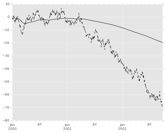
An expanding window statistic will be more stable (and less responsive) than its rolling window counterpart as the increasing window size decreases the relative impact of an individual data point. As an example, here is the mean() output for the previous time series dataset:
In [79]: s.plot(style='k--')
Out[79]: <matplotlib.axes._subplots.AxesSubplot at 0x118390f10>

In [80]: s.expanding().mean().plot(style='k')
Out[80]: <matplotlib.axes._subplots.AxesSubplot at 0x118390f10>
Exponentially Weighted Windows
A related set of functions are exponentially weighted versions of several of the above statistics. A similar interface to .rolling and .expanding is accessed thru the .ewm method to receive an EWM object. A number of expanding EW (exponentially weighted) methods are provided:
| Function | Description |
|---|---|
| mean() | EW moving average |
| var() | EW moving variance |
| std() | EW moving standard deviation |
| corr() | EW moving correlation |
| cov() | EW moving covariance |
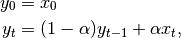
In general, a weighted moving average is calculated as
where  is the input and
  is the result.
The EW functions support two variants of exponential weights.
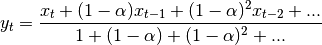
The default, adjust=True, uses the weights  which gives
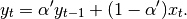
When adjust=False is specified, moving averages are calculated as
which is equivalent to using weights
Note
These equations are sometimes written in terms of  , e.g.
The difference between the above two variants arises because we are dealing with series which have finite history. Consider a series of infinite history:
Noting that the denominator is a geometric series with initial term equal to 1
and a ratio of  we have
![y_t &= \frac{x_t + (1 - \alpha)x_{t-1} + (1 - \alpha)^2 x_{t-2} + ...}
{\frac{1}{1 - (1 - \alpha)}}\\
&= [x_t + (1 - \alpha)x_{t-1} + (1 - \alpha)^2 x_{t-2} + ...] \alpha \\
&= \alpha x_t + [(1-\alpha)x_{t-1} + (1 - \alpha)^2 x_{t-2} + ...]\alpha \\
&= \alpha x_t + (1 - \alpha)[x_{t-1} + (1 - \alpha) x_{t-2} + ...]\alpha\\
&= \alpha x_t + (1 - \alpha) y_{t-1}](_images/math/2be73bffdf3cefb77c1cafd822ff2dafccd03a99.png)
which shows the equivalence of the above two variants for infinite series.
When adjust=True we have  and from the last
representation above we have
and from the last
representation above we have 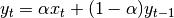 ,
therefore there is an assumption that
,
therefore there is an assumption that  is not an ordinary value
but rather an exponentially weighted moment of the infinite series up to that
point.
is not an ordinary value
but rather an exponentially weighted moment of the infinite series up to that
point.
One must have  , and while since version 0.18.0
it has been possible to pass
, and while since version 0.18.0
it has been possible to pass  directly, it’s often easier
to think about either the span, center of mass (com) or half-life
of an EW moment:
directly, it’s often easier
to think about either the span, center of mass (com) or half-life
of an EW moment:
One must specify precisely one of span, center of mass, half-life and alpha to the EW functions:
- Span corresponds to what is commonly called an “N-day EW moving average”.
- Center of mass has a more physical interpretation and can be thought of
in terms of span:
 .
. - Half-life is the period of time for the exponential weight to reduce to one half.
- Alpha specifies the smoothing factor directly.
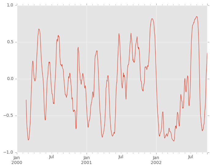
Here is an example for a univariate time series:
In [81]: s.plot(style='k--')
Out[81]: <matplotlib.axes._subplots.AxesSubplot at 0x1132e2dd0>

In [82]: s.ewm(span=20).mean().plot(style='k')
Out[82]: <matplotlib.axes._subplots.AxesSubplot at 0x1132e2dd0>
EWM has a min_periods argument, which has the same meaning it does for all the .expanding and .rolling methods: no output values will be set until at least min_periods non-null values are encountered in the (expanding) window. (This is a change from versions prior to 0.15.0, in which the min_periods argument affected only the min_periods consecutive entries starting at the first non-null value.)
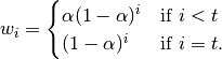
EWM also has an ignore_na argument, which deterines how intermediate null values affect the calculation of the weights. When ignore_na=False (the default), weights are calculated based on absolute positions, so that intermediate null values affect the result. When ignore_na=True (which reproduces the behavior in versions prior to 0.15.0), weights are calculated by ignoring intermediate null values. For example, assuming adjust=True, if ignore_na=False, the weighted average of 3, NaN, 5 would be calculated as
Whereas if ignore_na=True, the weighted average would be calculated as
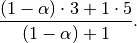
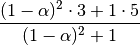
The var(), std(), and cov() functions have a bias argument, specifying whether the result should contain biased or unbiased statistics. For example, if bias=True, ewmvar(x) is calculated as ewmvar(x) = ewma(x**2) - ewma(x)**2; whereas if bias=False (the default), the biased variance statistics are scaled by debiasing factors
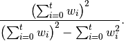
(For  , this reduces to the usual
  factor,
with
factor,
with  .)
See Weighted Sample Variance
for further details.
.)
See Weighted Sample Variance
for further details.