Scaling to large datasets#
pandas provides data structures for in-memory analytics, which makes using pandas to analyze datasets that are larger than memory datasets somewhat tricky. Even datasets that are a sizable fraction of memory become unwieldy, as some pandas operations need to make intermediate copies.
This document provides a few recommendations for scaling your analysis to larger datasets. It’s a complement to Enhancing performance, which focuses on speeding up analysis for datasets that fit in memory.
But first, it’s worth considering not using pandas. pandas isn’t the right tool for all situations. If you’re working with very large datasets and a tool like PostgreSQL fits your needs, then you should probably be using that. Assuming you want or need the expressiveness and power of pandas, let’s carry on.
Load less data#
Suppose our raw dataset on disk has many columns:
                     id_0    name_0       x_0       y_0  id_1   name_1       x_1  ...  name_8       x_8       y_8  id_9   name_9       x_9       y_9
timestamp                                                                         ...
2000-01-01 00:00:00  1015   Michael -0.399453  0.095427   994    Frank -0.176842  ...     Dan -0.315310  0.713892  1025   Victor -0.135779  0.346801
2000-01-01 00:01:00   969  Patricia  0.650773 -0.874275  1003    Laura  0.459153  ...  Ursula  0.913244 -0.630308  1047    Wendy -0.886285  0.035852
2000-01-01 00:02:00  1016    Victor -0.721465 -0.584710  1046  Michael  0.524994  ...     Ray -0.656593  0.692568  1064   Yvonne  0.070426  0.432047
2000-01-01 00:03:00   939     Alice -0.746004 -0.908008   996   Ingrid -0.414523  ...   Jerry -0.958994  0.608210   978    Wendy  0.855949 -0.648988
2000-01-01 00:04:00  1017       Dan  0.919451 -0.803504  1048    Jerry -0.569235  ...   Frank -0.577022 -0.409088   994      Bob -0.270132  0.335176
...                   ...       ...       ...       ...   ...      ...       ...  ...     ...       ...       ...   ...      ...       ...       ...
2000-12-30 23:56:00   999       Tim  0.162578  0.512817   973    Kevin -0.403352  ...     Tim -0.380415  0.008097  1041  Charlie  0.191477 -0.599519
2000-12-30 23:57:00   970     Laura -0.433586 -0.600289   958   Oliver -0.966577  ...   Zelda  0.971274  0.402032  1038   Ursula  0.574016 -0.930992
2000-12-30 23:58:00  1065     Edith  0.232211 -0.454540   971      Tim  0.158484  ...   Alice -0.222079 -0.919274  1022      Dan  0.031345 -0.657755
2000-12-30 23:59:00  1019    Ingrid  0.322208 -0.615974   981   Hannah  0.607517  ...   Sarah -0.424440 -0.117274   990   George -0.375530  0.563312
2000-12-31 00:00:00   937    Ursula -0.906523  0.943178  1018    Alice -0.564513  ...   Jerry  0.236837  0.807650   985   Oliver  0.777642  0.783392

[525601 rows x 40 columns]
That can be generated by the following code snippet:
In [1]: import pandas as pd

In [2]: import numpy as np

In [3]: def make_timeseries(start="2000-01-01", end="2000-12-31", freq="1D", seed=None):
   ...:     index = pd.date_range(start=start, end=end, freq=freq, name="timestamp")
   ...:     n = len(index)
   ...:     state = np.random.RandomState(seed)
   ...:     columns = {
   ...:         "name": state.choice(["Alice", "Bob", "Charlie"], size=n),
   ...:         "id": state.poisson(1000, size=n),
   ...:         "x": state.rand(n) * 2 - 1,
   ...:         "y": state.rand(n) * 2 - 1,
   ...:     }
   ...:     df = pd.DataFrame(columns, index=index, columns=sorted(columns))
   ...:     if df.index[-1] == end:
   ...:         df = df.iloc[:-1]
   ...:     return df
   ...:

In [4]: timeseries = [
   ...:     make_timeseries(freq="1T", seed=i).rename(columns=lambda x: f"{x}_{i}")
   ...:     for i in range(10)
   ...: ]
   ...:

In [5]: ts_wide = pd.concat(timeseries, axis=1)

In [6]: ts_wide.to_parquet("timeseries_wide.parquet")
To load the columns we want, we have two options. Option 1 loads in all the data and then filters to what we need.
In [7]: columns = ["id_0", "name_0", "x_0", "y_0"]

In [8]: pd.read_parquet("timeseries_wide.parquet")[columns]
Out[8]:
                     id_0 name_0       x_0       y_0
timestamp
2000-01-01 00:00:00   977  Alice -0.821225  0.906222
2000-01-01 00:01:00  1018    Bob -0.219182  0.350855
2000-01-01 00:02:00   927  Alice  0.660908 -0.798511
2000-01-01 00:03:00   997    Bob -0.852458  0.735260
2000-01-01 00:04:00   965    Bob  0.717283  0.393391
...                   ...    ...       ...       ...
2000-12-30 23:56:00  1037    Bob -0.814321  0.612836
2000-12-30 23:57:00   980    Bob  0.232195 -0.618828
2000-12-30 23:58:00   965  Alice -0.231131  0.026310
2000-12-30 23:59:00   984  Alice  0.942819  0.853128
2000-12-31 00:00:00  1003  Alice  0.201125 -0.136655

[525601 rows x 4 columns]
Option 2 only loads the columns we request.
In [9]: pd.read_parquet("timeseries_wide.parquet", columns=columns)
Out[9]:
                     id_0 name_0       x_0       y_0
timestamp
2000-01-01 00:00:00   977  Alice -0.821225  0.906222
2000-01-01 00:01:00  1018    Bob -0.219182  0.350855
2000-01-01 00:02:00   927  Alice  0.660908 -0.798511
2000-01-01 00:03:00   997    Bob -0.852458  0.735260
2000-01-01 00:04:00   965    Bob  0.717283  0.393391
...                   ...    ...       ...       ...
2000-12-30 23:56:00  1037    Bob -0.814321  0.612836
2000-12-30 23:57:00   980    Bob  0.232195 -0.618828
2000-12-30 23:58:00   965  Alice -0.231131  0.026310
2000-12-30 23:59:00   984  Alice  0.942819  0.853128
2000-12-31 00:00:00  1003  Alice  0.201125 -0.136655

[525601 rows x 4 columns]
If we were to measure the memory usage of the two calls, we’d see that specifying
columns uses about 1/10th the memory in this case.
With pandas.read_csv(), you can specify usecols to limit the columns
read into memory. Not all file formats that can be read by pandas provide an option
to read a subset of columns.
Use efficient datatypes#
The default pandas data types are not the most memory efficient. This is especially true for text data columns with relatively few unique values (commonly referred to as “low-cardinality” data). By using more efficient data types, you can store larger datasets in memory.
In [10]: ts = make_timeseries(freq="30S", seed=0)

In [11]: ts.to_parquet("timeseries.parquet")

In [12]: ts = pd.read_parquet("timeseries.parquet")

In [13]: ts
Out[13]:
                       id     name         x         y
timestamp
2000-01-01 00:00:00  1041    Alice  0.889987  0.281011
2000-01-01 00:00:30   988      Bob -0.455299  0.488153
2000-01-01 00:01:00  1018    Alice  0.096061  0.580473
2000-01-01 00:01:30   992      Bob  0.142482  0.041665
2000-01-01 00:02:00   960      Bob -0.036235  0.802159
...                   ...      ...       ...       ...
2000-12-30 23:58:00  1022    Alice  0.266191  0.875579
2000-12-30 23:58:30   974    Alice -0.009826  0.413686
2000-12-30 23:59:00  1028  Charlie  0.307108 -0.656789
2000-12-30 23:59:30  1002    Alice  0.202602  0.541335
2000-12-31 00:00:00   987    Alice  0.200832  0.615972

[1051201 rows x 4 columns]
Now, let’s inspect the data types and memory usage to see where we should focus our attention.
In [14]: ts.dtypes
Out[14]:
id        int64
name     object
x       float64
y       float64
dtype: object
In [15]: ts.memory_usage(deep=True)  # memory usage in bytes
Out[15]:
Index     8409608
id        8409608
name     65176434
x         8409608
y         8409608
dtype: int64
The name column is taking up much more memory than any other. It has just a
few unique values, so it’s a good candidate for converting to a
pandas.Categorical. With a pandas.Categorical, we store each unique name once and use
space-efficient integers to know which specific name is used in each row.
In [16]: ts2 = ts.copy()

In [17]: ts2["name"] = ts2["name"].astype("category")

In [18]: ts2.memory_usage(deep=True)
Out[18]:
Index    8409608
id       8409608
name     1051495
x        8409608
y        8409608
dtype: int64
We can go a bit further and downcast the numeric columns to their smallest types
using pandas.to_numeric().
In [19]: ts2["id"] = pd.to_numeric(ts2["id"], downcast="unsigned")

In [20]: ts2[["x", "y"]] = ts2[["x", "y"]].apply(pd.to_numeric, downcast="float")

In [21]: ts2.dtypes
Out[21]:
id        uint16
name    category
x        float32
y        float32
dtype: object
In [22]: ts2.memory_usage(deep=True)
Out[22]:
Index    8409608
id       2102402
name     1051495
x        4204804
y        4204804
dtype: int64
In [23]: reduction = ts2.memory_usage(deep=True).sum() / ts.memory_usage(deep=True).sum()

In [24]: print(f"{reduction:0.2f}")
0.20
In all, we’ve reduced the in-memory footprint of this dataset to 1/5 of its original size.
See Categorical data for more on pandas.Categorical and dtypes
for an overview of all of pandas’ dtypes.
Use chunking#
Some workloads can be achieved with chunking: splitting a large problem like “convert this directory of CSVs to parquet” into a bunch of small problems (“convert this individual CSV file into a Parquet file. Now repeat that for each file in this directory.”). As long as each chunk fits in memory, you can work with datasets that are much larger than memory.
Note
Chunking works well when the operation you’re performing requires zero or minimal coordination between chunks. For more complicated workflows, you’re better off using another library.
Suppose we have an even larger “logical dataset” on disk that’s a directory of parquet files. Each file in the directory represents a different year of the entire dataset.
In [25]: import pathlib

In [26]: N = 12

In [27]: starts = [f"20{i:>02d}-01-01" for i in range(N)]

In [28]: ends = [f"20{i:>02d}-12-13" for i in range(N)]

In [29]: pathlib.Path("data/timeseries").mkdir(exist_ok=True)

In [30]: for i, (start, end) in enumerate(zip(starts, ends)):
   ....:     ts = make_timeseries(start=start, end=end, freq="1T", seed=i)
   ....:     ts.to_parquet(f"data/timeseries/ts-{i:0>2d}.parquet")
   ....:
data
└── timeseries
    ├── ts-00.parquet
    ├── ts-01.parquet
    ├── ts-02.parquet
    ├── ts-03.parquet
    ├── ts-04.parquet
    ├── ts-05.parquet
    ├── ts-06.parquet
    ├── ts-07.parquet
    ├── ts-08.parquet
    ├── ts-09.parquet
    ├── ts-10.parquet
    └── ts-11.parquet
Now we’ll implement an out-of-core pandas.Series.value_counts(). The peak memory usage of this
workflow is the single largest chunk, plus a small series storing the unique value
counts up to this point. As long as each individual file fits in memory, this will
work for arbitrary-sized datasets.
In [31]: %%time
   ....: files = pathlib.Path("data/timeseries/").glob("ts*.parquet")
   ....: counts = pd.Series(dtype=int)
   ....: for path in files:
   ....:     df = pd.read_parquet(path)
   ....:     counts = counts.add(df["name"].value_counts(), fill_value=0)
   ....: counts.astype(int)
   ....:
CPU times: user 893 ms, sys: 91.5 ms, total: 984 ms
Wall time: 960 ms
Out[31]:
Alice      1994645
Bob        1993692
Charlie    1994875
dtype: int64
Some readers, like pandas.read_csv(), offer parameters to control the
chunksize when reading a single file.
Manually chunking is an OK option for workflows that don’t
require too sophisticated of operations. Some operations, like pandas.DataFrame.groupby(), are
much harder to do chunkwise. In these cases, you may be better switching to a
different library that implements these out-of-core algorithms for you.
Use other libraries#
pandas is just one library offering a DataFrame API. Because of its popularity, pandas’ API has become something of a standard that other libraries implement. The pandas documentation maintains a list of libraries implementing a DataFrame API in our ecosystem page.
For example, Dask, a parallel computing library, has dask.dataframe, a pandas-like API for working with larger than memory datasets in parallel. Dask can use multiple threads or processes on a single machine, or a cluster of machines to process data in parallel.
We’ll import dask.dataframe and notice that the API feels similar to pandas.
We can use Dask’s read_parquet function, but provide a globstring of files to read in.
In [32]: import dask.dataframe as dd

In [33]: ddf = dd.read_parquet("data/timeseries/ts*.parquet", engine="pyarrow")

In [34]: ddf
Out[34]:
Dask DataFrame Structure:
                   id    name        x        y
npartitions=12
                int64  object  float64  float64
                  ...     ...      ...      ...
...               ...     ...      ...      ...
                  ...     ...      ...      ...
                  ...     ...      ...      ...
Dask Name: read-parquet, 1 graph layer
Inspecting the ddf object, we see a few things
There are familiar attributes like
.columnsand.dtypesThere are familiar methods like
.groupby,.sum, etc.There are new attributes like
.npartitionsand.divisions
The partitions and divisions are how Dask parallelizes computation. A Dask
DataFrame is made up of many pandas pandas.DataFrame. A single method call on a
Dask DataFrame ends up making many pandas method calls, and Dask knows how to
coordinate everything to get the result.
In [35]: ddf.columns
Out[35]: Index(['id', 'name', 'x', 'y'], dtype='object')

In [36]: ddf.dtypes
Out[36]:
id        int64
name     object
x       float64
y       float64
dtype: object

In [37]: ddf.npartitions
Out[37]: 12
One major difference: the dask.dataframe API is lazy. If you look at the
repr above, you’ll notice that the values aren’t actually printed out; just the
column names and dtypes. That’s because Dask hasn’t actually read the data yet.
Rather than executing immediately, doing operations build up a task graph.
In [38]: ddf
Out[38]:
Dask DataFrame Structure:
                   id    name        x        y
npartitions=12
                int64  object  float64  float64
                  ...     ...      ...      ...
...               ...     ...      ...      ...
                  ...     ...      ...      ...
                  ...     ...      ...      ...
Dask Name: read-parquet, 1 graph layer

In [39]: ddf["name"]
Out[39]:
Dask Series Structure:
npartitions=12
    object
       ...
     ...
       ...
       ...
Name: name, dtype: object
Dask Name: getitem, 2 graph layers

In [40]: ddf["name"].value_counts()
Out[40]:
Dask Series Structure:
npartitions=1
    int64
      ...
Name: name, dtype: int64
Dask Name: value-counts-agg, 4 graph layers
Each of these calls is instant because the result isn’t being computed yet.
We’re just building up a list of computation to do when someone needs the
result. Dask knows that the return type of a pandas.Series.value_counts
is a pandas pandas.Series with a certain dtype and a certain name. So the Dask version
returns a Dask Series with the same dtype and the same name.
To get the actual result you can call .compute().
In [41]: %time ddf["name"].value_counts().compute()
CPU times: user 914 ms, sys: 28.6 ms, total: 943 ms
Wall time: 931 ms
Out[41]:
Charlie    1994875
Alice      1994645
Bob        1993692
Name: name, dtype: int64
At that point, you get back the same thing you’d get with pandas, in this case
a concrete pandas pandas.Series with the count of each name.
Calling .compute causes the full task graph to be executed. This includes
reading the data, selecting the columns, and doing the value_counts. The
execution is done in parallel where possible, and Dask tries to keep the
overall memory footprint small. You can work with datasets that are much larger
than memory, as long as each partition (a regular pandas pandas.DataFrame) fits in memory.
By default, dask.dataframe operations use a threadpool to do operations in
parallel. We can also connect to a cluster to distribute the work on many
machines. In this case we’ll connect to a local “cluster” made up of several
processes on this single machine.
>>> from dask.distributed import Client, LocalCluster

>>> cluster = LocalCluster()
>>> client = Client(cluster)
>>> client
<Client: 'tcp://127.0.0.1:53349' processes=4 threads=8, memory=17.18 GB>
Once this client is created, all of Dask’s computation will take place on
the cluster (which is just processes in this case).
Dask implements the most used parts of the pandas API. For example, we can do a familiar groupby aggregation.
In [42]: %time ddf.groupby("name")[["x", "y"]].mean().compute().head()
CPU times: user 2.04 s, sys: 119 ms, total: 2.16 s
Wall time: 1.99 s
Out[42]:
                x         y
name
Alice   -0.000224 -0.000194
Bob     -0.000746  0.000349
Charlie  0.000604  0.000250
The grouping and aggregation is done out-of-core and in parallel.
When Dask knows the divisions of a dataset, certain optimizations are
possible. When reading parquet datasets written by dask, the divisions will be
known automatically. In this case, since we created the parquet files manually,
we need to supply the divisions manually.
In [43]: N = 12

In [44]: starts = [f"20{i:>02d}-01-01" for i in range(N)]

In [45]: ends = [f"20{i:>02d}-12-13" for i in range(N)]

In [46]: divisions = tuple(pd.to_datetime(starts)) + (pd.Timestamp(ends[-1]),)

In [47]: ddf.divisions = divisions

In [48]: ddf
Out[48]:
Dask DataFrame Structure:
                   id    name        x        y
npartitions=12
2000-01-01      int64  object  float64  float64
2001-01-01        ...     ...      ...      ...
...               ...     ...      ...      ...
2011-01-01        ...     ...      ...      ...
2011-12-13        ...     ...      ...      ...
Dask Name: read-parquet, 1 graph layer
Now we can do things like fast random access with .loc.
In [49]: ddf.loc["2002-01-01 12:01":"2002-01-01 12:05"].compute()
Out[49]:
                       id     name         x         y
timestamp
2002-01-01 12:01:00   971      Bob -0.659481  0.556184
2002-01-01 12:02:00  1015  Charlie  0.120131 -0.609522
2002-01-01 12:03:00   991      Bob -0.357816  0.811362
2002-01-01 12:04:00   984    Alice -0.608760  0.034187
2002-01-01 12:05:00   998  Charlie  0.551662 -0.461972
Dask knows to just look in the 3rd partition for selecting values in 2002. It doesn’t need to look at any other data.
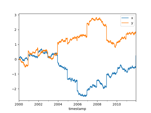
Many workflows involve a large amount of data and processing it in a way that
reduces the size to something that fits in memory. In this case, we’ll resample
to daily frequency and take the mean. Once we’ve taken the mean, we know the
results will fit in memory, so we can safely call compute without running
out of memory. At that point it’s just a regular pandas object.
In [50]: ddf[["x", "y"]].resample("1D").mean().cumsum().compute().plot()
Out[50]: <AxesSubplot: xlabel='timestamp'>
These Dask examples have all be done using multiple processes on a single machine. Dask can be deployed on a cluster to scale up to even larger datasets.
You see more dask examples at https://examples.dask.org.