Frequently Asked Questions (FAQ)
DataFrame memory usage
As of pandas version 0.15.0, the memory usage of a dataframe (including the index) is shown when accessing the info method of a dataframe. A configuration option, display.memory_usage (see Options and Settings), specifies if the dataframe’s memory usage will be displayed when invoking the df.info() method.
For example, the memory usage of the dataframe below is shown when calling df.info():
In [1]: dtypes = ['int64', 'float64', 'datetime64[ns]', 'timedelta64[ns]',
   ...:            'complex128', 'object', 'bool']
   ...:

In [2]: n = 5000

In [3]: data = dict([ (t, np.random.randint(100, size=n).astype(t))
   ...:                 for t in dtypes])
   ...:

In [4]: df = DataFrame(data)

In [5]: df['categorical'] = df['object'].astype('category')

In [6]: df.info()
<class 'pandas.core.frame.DataFrame'>
Int64Index: 5000 entries, 0 to 4999
Data columns (total 8 columns):
bool               5000 non-null bool
complex128         5000 non-null complex128
datetime64[ns]     5000 non-null datetime64[ns]
float64            5000 non-null float64
int64              5000 non-null int64
object             5000 non-null object
timedelta64[ns]    5000 non-null timedelta64[ns]
categorical        5000 non-null category
dtypes: bool(1), category(1), complex128(1), datetime64[ns](1), float64(1), int64(1), object(1), timedelta64[ns](1)
memory usage: 303.5+ KB
The + symbol indicates that the true memory usage could be higher, because pandas does not count the memory used by values in columns with dtype=object.
By default the display option is set to True but can be explicitly overridden by passing the memory_usage argument when invoking df.info().
The memory usage of each column can be found by calling the memory_usage method. This returns a Series with an index represented by column names and memory usage of each column shown in bytes. For the dataframe above, the memory usage of each column and the total memory usage of the dataframe can be found with the memory_usage method:
In [7]: df.memory_usage()
Out[7]:
bool                5000
complex128         80000
datetime64[ns]     40000
float64            40000
int64              40000
object             20000
timedelta64[ns]    40000
categorical         5800
dtype: int64

# total memory usage of dataframe
In [8]: df.memory_usage().sum()
Out[8]: 270800
By default the memory usage of the dataframe’s index is not shown in the returned Series, the memory usage of the index can be shown by passing the index=True argument:
In [9]: df.memory_usage(index=True)
Out[9]:
Index              40000
bool                5000
complex128         80000
datetime64[ns]     40000
float64            40000
int64              40000
object             20000
timedelta64[ns]    40000
categorical         5800
dtype: int64
The memory usage displayed by the info method utilizes the memory_usage method to determine the memory usage of a dataframe while also formatting the output in human-readable units (base-2 representation; i.e., 1KB = 1024 bytes).
See also Categorical Memory Usage.
Adding Features to your pandas Installation
pandas is a powerful tool and already has a plethora of data manipulation operations implemented, most of them are very fast as well. It’s very possible however that certain functionality that would make your life easier is missing. In that case you have several options:
Open an issue on Github , explain your need and the sort of functionality you would like to see implemented.
Fork the repo, Implement the functionality yourself and open a PR on Github.
Write a method that performs the operation you are interested in and Monkey-patch the pandas class as part of your IPython profile startup or PYTHONSTARTUP file.
For example, here is an example of adding an just_foo_cols() method to the dataframe class:
import pandas as pd
def just_foo_cols(self):
    """Get a list of column names containing the string 'foo'

    """
    return [x for x in self.columns if 'foo' in x]

pd.DataFrame.just_foo_cols = just_foo_cols # monkey-patch the DataFrame class
df = pd.DataFrame([list(range(4))], columns=["A","foo","foozball","bar"])
df.just_foo_cols()
del pd.DataFrame.just_foo_cols # you can also remove the new method
Monkey-patching is usually frowned upon because it makes your code less portable and can cause subtle bugs in some circumstances. Monkey-patching existing methods is usually a bad idea in that respect. When used with proper care, however, it’s a very useful tool to have.
Migrating from scikits.timeseries to pandas >= 0.8.0
Starting with pandas 0.8.0, users of scikits.timeseries should have all of the features that they need to migrate their code to use pandas. Portions of the scikits.timeseries codebase for implementing calendar logic and timespan frequency conversions (but not resampling, that has all been implemented from scratch from the ground up) have been ported to the pandas codebase.
The scikits.timeseries notions of Date and DateArray are responsible for implementing calendar logic:
In [16]: dt = ts.Date('Q', '1984Q3')

# sic
In [17]: dt
Out[17]: <Q-DEC : 1984Q1>

In [18]: dt.asfreq('D', 'start')
Out[18]: <D : 01-Jan-1984>

In [19]: dt.asfreq('D', 'end')
Out[19]: <D : 31-Mar-1984>

In [20]: dt + 3
Out[20]: <Q-DEC : 1984Q4>
Date and DateArray from scikits.timeseries have been reincarnated in pandas Period and PeriodIndex:
In [10]: pnow('D')  # scikits.timeseries.now()
Out[10]: Period('2015-05-11', 'D')

In [11]: Period(year=2007, month=3, day=15, freq='D')
Out[11]: Period('2007-03-15', 'D')

In [12]: p = Period('1984Q3')

In [13]: p
Out[13]: Period('1984Q3', 'Q-DEC')

In [14]: p.asfreq('D', 'start')
Out[14]: Period('1984-07-01', 'D')

In [15]: p.asfreq('D', 'end')
Out[15]: Period('1984-09-30', 'D')

In [16]: (p + 3).asfreq('T') + 6 * 60 + 30
Out[16]: Period('1985-07-01 06:29', 'T')

In [17]: rng = period_range('1990', '2010', freq='A')

In [18]: rng
Out[18]:
PeriodIndex(['1990', '1991', '1992', '1993', '1994', '1995', '1996', '1997',
             '1998', '1999', '2000', '2001', '2002', '2003', '2004', '2005',
             '2006', '2007', '2008', '2009', '2010'],
            dtype='int64', freq='A-DEC')

In [19]: rng.asfreq('B', 'end') - 3
Out[19]:
PeriodIndex(['1990-12-26', '1991-12-26', '1992-12-28', '1993-12-28',
             '1994-12-27', '1995-12-26', '1996-12-26', '1997-12-26',
             '1998-12-28', '1999-12-28', '2000-12-26', '2001-12-26',
             '2002-12-26', '2003-12-26', '2004-12-28', '2005-12-27',
             '2006-12-26', '2007-12-26', '2008-12-26', '2009-12-28',
             '2010-12-28'],
            dtype='int64', freq='B')
| scikits.timeseries | pandas | Notes |
|---|---|---|
| Date | Period | A span of time, from yearly through to secondly |
| DateArray | PeriodIndex | An array of timespans |
| convert | resample | Frequency conversion in scikits.timeseries |
| convert_to_annual | pivot_annual | currently supports up to daily frequency, see GH736 |
PeriodIndex / DateArray properties and functions
The scikits.timeseries DateArray had a number of information properties. Here are the pandas equivalents:
| scikits.timeseries | pandas | Notes |
|---|---|---|
| get_steps | np.diff(idx.values) | |
| has_missing_dates | not idx.is_full | |
| is_full | idx.is_full | |
| is_valid | idx.is_monotonic and idx.is_unique | |
| is_chronological | is_monotonic | |
| arr.sort_chronologically() | idx.order() |
Frequency conversion
Frequency conversion is implemented using the resample method on TimeSeries and DataFrame objects (multiple time series). resample also works on panels (3D). Here is some code that resamples daily data to monthly:
In [20]: rng = period_range('Jan-2000', periods=50, freq='M')

In [21]: data = Series(np.random.randn(50), index=rng)

In [22]: data
Out[22]:
2000-01    1.544821
2000-02   -1.708552
2000-03    1.545458
2000-04   -0.735738
2000-05   -0.649091
2000-06   -0.403878
2000-07   -2.474932
             ...
2003-08    1.034493
2003-09    1.269838
2003-10    0.606166
2003-11   -0.827409
2003-12   -0.943863
2004-01    1.041569
2004-02    0.701815
Freq: M, dtype: float64

In [23]: data.resample('A', how=np.mean)
Out[23]:
2000    0.102447
2001   -0.204847
2002    0.210840
2003    0.300564
2004    0.871692
Freq: A-DEC, dtype: float64
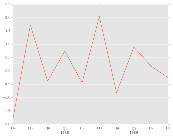
Plotting
Much of the plotting functionality of scikits.timeseries has been ported and adopted to pandas’s data structures. For example:
In [24]: rng = period_range('1987Q2', periods=10, freq='Q-DEC')

In [25]: data = Series(np.random.randn(10), index=rng)

In [26]: plt.figure(); data.plot()
Out[26]: <matplotlib.axes._subplots.AxesSubplot at 0xa18186cc>
Converting to and from period format
Use the to_timestamp and to_period instance methods.
Treatment of missing data
Unlike scikits.timeseries, pandas data structures are not based on NumPy’s MaskedArray object. Missing data is represented as NaN in numerical arrays and either as None or NaN in non-numerical arrays. Implementing a version of pandas’s data structures that use MaskedArray is possible but would require the involvement of a dedicated maintainer. Active pandas developers are not interested in this.
Resampling with timestamps and periods
resample has a kind argument which allows you to resample time series with a DatetimeIndex to PeriodIndex:
In [27]: rng = date_range('1/1/2000', periods=200, freq='D')

In [28]: data = Series(np.random.randn(200), index=rng)

In [29]: data[:10]
Out[29]:
2000-01-01   -0.197661
2000-01-02    0.507155
2000-01-03   -0.493913
2000-01-04   -0.994339
2000-01-05   -0.581662
2000-01-06   -0.855251
2000-01-07   -0.256469
2000-01-08   -0.454868
2000-01-09    0.519612
2000-01-10    0.764490
Freq: D, dtype: float64

In [30]: data.index
Out[30]:
DatetimeIndex(['2000-01-01', '2000-01-02', '2000-01-03', '2000-01-04',
               '2000-01-05', '2000-01-06', '2000-01-07', '2000-01-08',
               '2000-01-09', '2000-01-10',
               ...
               '2000-07-09', '2000-07-10', '2000-07-11', '2000-07-12',
               '2000-07-13', '2000-07-14', '2000-07-15', '2000-07-16',
               '2000-07-17', '2000-07-18'],
              dtype='datetime64[ns]', length=200, freq='D', tz=None)

In [31]: data.resample('M', kind='period')
Out[31]:
2000-01   -0.226155
2000-02    0.056704
2000-03   -0.132553
2000-04   -0.064003
2000-05    0.233736
2000-06   -0.301008
2000-07   -0.584631
Freq: M, dtype: float64
Similarly, resampling from periods to timestamps is possible with an optional interval ('start' or 'end') convention:
In [32]: rng = period_range('Jan-2000', periods=50, freq='M')

In [33]: data = Series(np.random.randn(50), index=rng)

In [34]: resampled = data.resample('A', kind='timestamp', convention='end')

In [35]: resampled.index
Out[35]:
DatetimeIndex(['2000-12-31', '2001-12-31', '2002-12-31', '2003-12-31',
               '2004-12-31'],
              dtype='datetime64[ns]', freq='A-DEC', tz=None)
Byte-Ordering Issues
Occasionally you may have to deal with data that were created on a machine with a different byte order than the one on which you are running Python. To deal with this issue you should convert the underlying NumPy array to the native system byte order before passing it to Series/DataFrame/Panel constructors using something similar to the following:
In [36]: x = np.array(list(range(10)), '>i4') # big endian

In [37]: newx = x.byteswap().newbyteorder() # force native byteorder

In [38]: s = Series(newx)
See the NumPy documentation on byte order for more details.
Visualizing Data in Qt applications
Warning
The qt support is deprecated and will be removed in a future version. We refer users to the external package pandas-qt.
There is experimental support for visualizing DataFrames in PyQt4 and PySide applications. At the moment you can display and edit the values of the cells in the DataFrame. Qt will take care of displaying just the portion of the DataFrame that is currently visible and the edits will be immediately saved to the underlying DataFrame
To demonstrate this we will create a simple PySide application that will switch between two editable DataFrames. For this will use the DataFrameModel class that handles the access to the DataFrame, and the DataFrameWidget, which is just a thin layer around the QTableView.
import numpy as np
import pandas as pd
from pandas.sandbox.qtpandas import DataFrameModel, DataFrameWidget
from PySide import QtGui, QtCore

# Or if you use PyQt4:
# from PyQt4 import QtGui, QtCore

class MainWidget(QtGui.QWidget):
    def __init__(self, parent=None):
        super(MainWidget, self).__init__(parent)

        # Create two DataFrames
        self.df1 = pd.DataFrame(np.arange(9).reshape(3, 3),
                                columns=['foo', 'bar', 'baz'])
        self.df2 = pd.DataFrame({
                'int': [1, 2, 3],
                'float': [1.5, 2.5, 3.5],
                'string': ['a', 'b', 'c'],
                'nan': [np.nan, np.nan, np.nan]
            }, index=['AAA', 'BBB', 'CCC'],
            columns=['int', 'float', 'string', 'nan'])

        # Create the widget and set the first DataFrame
        self.widget = DataFrameWidget(self.df1)

        # Create the buttons for changing DataFrames
        self.button_first = QtGui.QPushButton('First')
        self.button_first.clicked.connect(self.on_first_click)
        self.button_second = QtGui.QPushButton('Second')
        self.button_second.clicked.connect(self.on_second_click)

        # Set the layout
        vbox = QtGui.QVBoxLayout()
        vbox.addWidget(self.widget)
        hbox = QtGui.QHBoxLayout()
        hbox.addWidget(self.button_first)
        hbox.addWidget(self.button_second)
        vbox.addLayout(hbox)
        self.setLayout(vbox)

    def on_first_click(self):
        '''Sets the first DataFrame'''
        self.widget.setDataFrame(self.df1)

    def on_second_click(self):
        '''Sets the second DataFrame'''
        self.widget.setDataFrame(self.df2)

if __name__ == '__main__':
    import sys

    # Initialize the application
    app = QtGui.QApplication(sys.argv)
    mw = MainWidget()
    mw.show()
    app.exec_()