

In [1]: import pandas as pd
- Titanic data
This tutorial uses the Titanic data set, stored as CSV. The data consists of the following data columns:
PassengerId: Id of every passenger.
Survived: Indication whether passenger survived.
0for no and1for yes.Pclass: One out of the 3 ticket classes: Class
1, Class2and Class3.Name: Name of passenger.
Sex: Gender of passenger.
Age: Age of passenger in years.
SibSp: Number of siblings or spouses aboard.
Parch: Number of parents or children aboard.
Ticket: Ticket number of passenger.
Fare: Indicating the fare.
Cabin: Cabin number of passenger.
Embarked: Port of embarkation.
In [2]: titanic = pd.read_csv("data/titanic.csv")

In [3]: titanic.head()
Out[3]:
   PassengerId  Survived  Pclass  ...     Fare Cabin Embarked
0            1         0       3  ...   7.2500   NaN        S
1            2         1       1  ...  71.2833   C85        C
2            3         1       3  ...   7.9250   NaN        S
3            4         1       1  ...  53.1000  C123        S
4            5         0       3  ...   8.0500   NaN        S

[5 rows x 12 columns]
-
Air quality data
This tutorial uses air quality data about \(NO_2\) and Particulate matter less than 2.5 micrometers, made available by OpenAQ and using the py-openaq package. The
air_quality_long.csvdata set provides \(NO_2\) and \(PM_{25}\) values for the measurement stations FR04014, BETR801 and London Westminster in respectively Paris, Antwerp and London.The air-quality data set has the following columns:
city: city where the sensor is used, either Paris, Antwerp or London
country: country where the sensor is used, either FR, BE or GB
location: the id of the sensor, either FR04014, BETR801 or London Westminster
parameter: the parameter measured by the sensor, either \(NO_2\) or Particulate matter
value: the measured value
unit: the unit of the measured parameter, in this case ‘µg/m³’
and the index of the
DataFrameisdatetime, the datetime of the measurement.To raw dataNote
The air-quality data is provided in a so-called long format data representation with each observation on a separate row and each variable a separate column of the data table. The long/narrow format is also known as the tidy data format.
In [4]: air_quality = pd.read_csv(
   ...:     "data/air_quality_long.csv", index_col="date.utc", parse_dates=True
   ...: )
   ...:

In [5]: air_quality.head()
Out[5]:
                                city country location parameter  value   unit
date.utc
2019-06-18 06:00:00+00:00  Antwerpen      BE  BETR801      pm25   18.0  µg/m³
2019-06-17 08:00:00+00:00  Antwerpen      BE  BETR801      pm25    6.5  µg/m³
2019-06-17 07:00:00+00:00  Antwerpen      BE  BETR801      pm25   18.5  µg/m³
2019-06-17 06:00:00+00:00  Antwerpen      BE  BETR801      pm25   16.0  µg/m³
2019-06-17 05:00:00+00:00  Antwerpen      BE  BETR801      pm25    7.5  µg/m³
How to reshape the layout of tables#
Sort table rows#
I want to sort the Titanic data according to the age of the passengers.
In [6]: titanic.sort_values(by="Age").head()
Out[6]:
     PassengerId  Survived  Pclass  ...     Fare Cabin Embarked
803          804         1       3  ...   8.5167   NaN        C
755          756         1       2  ...  14.5000   NaN        S
644          645         1       3  ...  19.2583   NaN        C
469          470         1       3  ...  19.2583   NaN        C
78            79         1       2  ...  29.0000   NaN        S

[5 rows x 12 columns]
I want to sort the Titanic data according to the cabin class and age in descending order.
In [7]: titanic.sort_values(by=['Pclass', 'Age'], ascending=False).head()
Out[7]:
     PassengerId  Survived  Pclass  ...    Fare Cabin Embarked
851          852         0       3  ...  7.7750   NaN        S
116          117         0       3  ...  7.7500   NaN        Q
280          281         0       3  ...  7.7500   NaN        Q
483          484         1       3  ...  9.5875   NaN        S
326          327         0       3  ...  6.2375   NaN        S

[5 rows x 12 columns]
With
DataFrame.sort_values(), the rows in the table are sorted according to the defined column(s). The index will follow the row order.
More details about sorting of tables is provided in the user guide section on sorting data.
Long to wide table format#
Let’s use a small subset of the air quality data set. We focus on
\(NO_2\) data and only use the first two measurements of each
location (i.e. the head of each group). The subset of data will be
called no2_subset.
# filter for no2 data only
In [8]: no2 = air_quality[air_quality["parameter"] == "no2"]
# use 2 measurements (head) for each location (groupby)
In [9]: no2_subset = no2.sort_index().groupby(["location"]).head(2)

In [10]: no2_subset
Out[10]:
                                city country  ...  value   unit
date.utc                                      ...
2019-04-09 01:00:00+00:00  Antwerpen      BE  ...   22.5  µg/m³
2019-04-09 01:00:00+00:00      Paris      FR  ...   24.4  µg/m³
2019-04-09 02:00:00+00:00     London      GB  ...   67.0  µg/m³
2019-04-09 02:00:00+00:00  Antwerpen      BE  ...   53.5  µg/m³
2019-04-09 02:00:00+00:00      Paris      FR  ...   27.4  µg/m³
2019-04-09 03:00:00+00:00     London      GB  ...   67.0  µg/m³

[6 rows x 6 columns]

I want the values for the three stations as separate columns next to each other.
In [11]: no2_subset.pivot(columns="location", values="value")
Out[11]:
location                   BETR801  FR04014  London Westminster
date.utc
2019-04-09 01:00:00+00:00     22.5     24.4                 NaN
2019-04-09 02:00:00+00:00     53.5     27.4                67.0
2019-04-09 03:00:00+00:00      NaN      NaN                67.0
The
pivot()function is purely reshaping of the data: a single value for each index/column combination is required.
As pandas supports plotting of multiple columns (see plotting tutorial) out of the box, the conversion from long to wide table format enables the plotting of the different time series at the same time:
In [12]: no2.head()
Out[12]:
                            city country location parameter  value   unit
date.utc
2019-06-21 00:00:00+00:00  Paris      FR  FR04014       no2   20.0  µg/m³
2019-06-20 23:00:00+00:00  Paris      FR  FR04014       no2   21.8  µg/m³
2019-06-20 22:00:00+00:00  Paris      FR  FR04014       no2   26.5  µg/m³
2019-06-20 21:00:00+00:00  Paris      FR  FR04014       no2   24.9  µg/m³
2019-06-20 20:00:00+00:00  Paris      FR  FR04014       no2   21.4  µg/m³
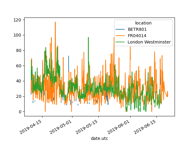
In [13]: no2.pivot(columns="location", values="value").plot()
Out[13]: <Axes: xlabel='date.utc'>
Note
When the index parameter is not defined, the existing
index (row labels) is used.
For more information about pivot(), see the user guide section on pivoting DataFrame objects.
Pivot table#

I want the mean concentrations for \(NO_2\) and \(PM_{2.5}\) in each of the stations in table form.
In [14]: air_quality.pivot_table(
   ....:     values="value", index="location", columns="parameter", aggfunc="mean"
   ....: )
   ....:
Out[14]:
parameter                 no2       pm25
location
BETR801             26.950920  23.169492
FR04014             29.374284        NaN
London Westminster  29.740050  13.443568
In the case of
pivot(), the data is only rearranged. When multiple values need to be aggregated (in this specific case, the values on different time steps),pivot_table()can be used, providing an aggregation function (e.g. mean) on how to combine these values.
Pivot table is a well known concept in spreadsheet software. When
interested in the row/column margins (subtotals) for each variable, set
the margins parameter to True:
In [15]: air_quality.pivot_table(
   ....:     values="value",
   ....:     index="location",
   ....:     columns="parameter",
   ....:     aggfunc="mean",
   ....:     margins=True,
   ....: )
   ....:
Out[15]:
parameter                 no2       pm25        All
location
BETR801             26.950920  23.169492  24.982353
FR04014             29.374284        NaN  29.374284
London Westminster  29.740050  13.443568  21.491708
All                 29.430316  14.386849  24.222743
For more information about pivot_table(), see the user guide section on pivot tables.
Note
In case you are wondering, pivot_table() is indeed directly linked
to groupby(). The same result can be derived by grouping on both
parameter and location:
air_quality.groupby(["parameter", "location"])[["value"]].mean()
Wide to long format#
Starting again from the wide format table created in the previous
section, we add a new index to the DataFrame with reset_index().
In [16]: no2_pivoted = no2.pivot(columns="location", values="value").reset_index()

In [17]: no2_pivoted.head()
Out[17]:
location                  date.utc  BETR801  FR04014  London Westminster
0        2019-04-09 01:00:00+00:00     22.5     24.4                 NaN
1        2019-04-09 02:00:00+00:00     53.5     27.4                67.0
2        2019-04-09 03:00:00+00:00     54.5     34.2                67.0
3        2019-04-09 04:00:00+00:00     34.5     48.5                41.0
4        2019-04-09 05:00:00+00:00     46.5     59.5                41.0

I want to collect all air quality \(NO_2\) measurements in a single column (long format).
In [18]: no_2 = no2_pivoted.melt(id_vars="date.utc")

In [19]: no_2.head()
Out[19]:
                   date.utc location  value
0 2019-04-09 01:00:00+00:00  BETR801   22.5
1 2019-04-09 02:00:00+00:00  BETR801   53.5
2 2019-04-09 03:00:00+00:00  BETR801   54.5
3 2019-04-09 04:00:00+00:00  BETR801   34.5
4 2019-04-09 05:00:00+00:00  BETR801   46.5
The
pandas.melt()method on aDataFrameconverts the data table from wide format to long format. The column headers become the variable names in a newly created column.
The solution is the short version on how to apply pandas.melt(). The method
will melt all columns NOT mentioned in id_vars together into two
columns: A column with the column header names and a column with the
values itself. The latter column gets by default the name value.
The parameters passed to pandas.melt() can be defined in more detail:
In [20]: no_2 = no2_pivoted.melt(
   ....:     id_vars="date.utc",
   ....:     value_vars=["BETR801", "FR04014", "London Westminster"],
   ....:     value_name="NO_2",
   ....:     var_name="id_location",
   ....: )
   ....:

In [21]: no_2.head()
Out[21]:
                   date.utc id_location  NO_2
0 2019-04-09 01:00:00+00:00     BETR801  22.5
1 2019-04-09 02:00:00+00:00     BETR801  53.5
2 2019-04-09 03:00:00+00:00     BETR801  54.5
3 2019-04-09 04:00:00+00:00     BETR801  34.5
4 2019-04-09 05:00:00+00:00     BETR801  46.5
The additional parameters have the following effects:
value_varsdefines which columns to melt togethervalue_nameprovides a custom column name for the values column instead of the default column namevaluevar_nameprovides a custom column name for the column collecting the column header names. Otherwise it takes the index name or a defaultvariable
Hence, the arguments value_name and var_name are just
user-defined names for the two generated columns. The columns to melt
are defined by id_vars and value_vars.
Conversion from wide to long format with pandas.melt() is explained in the user guide section on reshaping by melt.
REMEMBER
Sorting by one or more columns is supported by
sort_values.The
pivotfunction is purely restructuring of the data,pivot_tablesupports aggregations.The reverse of
pivot(long to wide format) ismelt(wide to long format).
A full overview is available in the user guide on the pages about reshaping and pivoting.