

Reshaping and pivot tables#
pandas provides methods for manipulating a Series and DataFrame to alter the
representation of the data for further data processing or data summarization.
pivot()andpivot_table(): Group unique values within one or more discrete categories.stack()andunstack(): Pivot a column or row level to the opposite axis respectively.melt()andwide_to_long(): Unpivot a wideDataFrameto a long format.get_dummies()andfrom_dummies(): Conversions with indicator variables.explode(): Convert a column of list-like values to individual rows.crosstab(): Calculate a cross-tabulation of multiple 1 dimensional factor arrays.cut(): Transform continuous variables to discrete, categorical valuesfactorize(): Encode 1 dimensional variables into integer labels.
pivot() and pivot_table()#
pivot()#
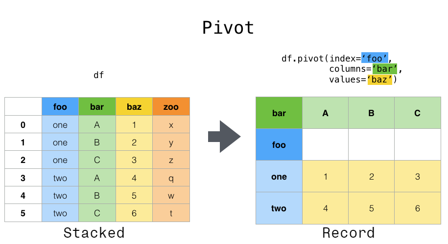
Data is often stored in so-called “stacked” or “record” format. In a “record” or “wide” format, typically there is one row for each subject. In the “stacked” or “long” format there are multiple rows for each subject where applicable.
In [1]: data = {
   ...:    "value": range(12),
   ...:    "variable": ["A"] * 3 + ["B"] * 3 + ["C"] * 3 + ["D"] * 3,
   ...:    "date": pd.to_datetime(["2020-01-03", "2020-01-04", "2020-01-05"] * 4)
   ...: }
   ...:

In [2]: df = pd.DataFrame(data)
To perform time series operations with each unique variable, a better
representation would be where the columns are the unique variables and an
index of dates identifies individual observations. To reshape the data into
this form, we use the DataFrame.pivot() method (also implemented as a
top level function pivot()):
In [3]: pivoted = df.pivot(index="date", columns="variable", values="value")

In [4]: pivoted
Out[4]:
variable    A  B  C   D
date
2020-01-03  0  3  6   9
2020-01-04  1  4  7  10
2020-01-05  2  5  8  11
If the values argument is omitted, and the input DataFrame has more than
one column of values which are not used as column or index inputs to pivot(),
then the resulting “pivoted” DataFrame will have hierarchical columns whose topmost level indicates the respective value
column:
In [5]: df["value2"] = df["value"] * 2

In [6]: pivoted = df.pivot(index="date", columns="variable")

In [7]: pivoted
Out[7]:
           value           value2
variable       A  B  C   D      A   B   C   D
date
2020-01-03     0  3  6   9      0   6  12  18
2020-01-04     1  4  7  10      2   8  14  20
2020-01-05     2  5  8  11      4  10  16  22
You can then select subsets from the pivoted DataFrame:
In [8]: pivoted["value2"]
Out[8]:
variable    A   B   C   D
date
2020-01-03  0   6  12  18
2020-01-04  2   8  14  20
2020-01-05  4  10  16  22
Note that this returns a view on the underlying data in the case where the data are homogeneously-typed.
Note
pivot() can only handle unique rows specified by index and columns.
If your data contains duplicates, use pivot_table().
pivot_table()#
While pivot() provides general purpose pivoting with various
data types, pandas also provides pivot_table() or pivot_table()
for pivoting with aggregation of numeric data.
The function pivot_table() can be used to create spreadsheet-style
pivot tables. See the cookbook for some advanced
strategies.
In [9]: import datetime

In [10]: df = pd.DataFrame(
   ....:     {
   ....:         "A": ["one", "one", "two", "three"] * 6,
   ....:         "B": ["A", "B", "C"] * 8,
   ....:         "C": ["foo", "foo", "foo", "bar", "bar", "bar"] * 4,
   ....:         "D": np.random.randn(24),
   ....:         "E": np.random.randn(24),
   ....:         "F": [datetime.datetime(2013, i, 1) for i in range(1, 13)]
   ....:         + [datetime.datetime(2013, i, 15) for i in range(1, 13)],
   ....:     }
   ....: )
   ....:

In [11]: df
Out[11]:
        A  B    C         D         E          F
0     one  A  foo  0.469112  0.404705 2013-01-01
1     one  B  foo -0.282863  0.577046 2013-02-01
2     two  C  foo -1.509059 -1.715002 2013-03-01
3   three  A  bar -1.135632 -1.039268 2013-04-01
4     one  B  bar  1.212112 -0.370647 2013-05-01
..    ... ..  ...       ...       ...        ...
19  three  B  foo -1.087401 -0.472035 2013-08-15
20    one  C  foo -0.673690 -0.013960 2013-09-15
21    one  A  bar  0.113648 -0.362543 2013-10-15
22    two  B  bar -1.478427 -0.006154 2013-11-15
23  three  C  bar  0.524988 -0.923061 2013-12-15

[24 rows x 6 columns]

In [12]: pd.pivot_table(df, values="D", index=["A", "B"], columns=["C"])
Out[12]:
C             bar       foo
A     B
one   A -0.995460  0.595334
      B  0.393570 -0.494817
      C  0.196903 -0.767769
three A -0.431886       NaN
      B       NaN -1.065818
      C  0.798396       NaN
two   A       NaN  0.197720
      B -0.986678       NaN
      C       NaN -1.274317

In [13]: pd.pivot_table(
   ....:     df, values=["D", "E"],
   ....:     index=["B"],
   ....:     columns=["A", "C"],
   ....:     aggfunc="sum",
   ....: )
   ....:
Out[13]:
          D                      ...
A       one               three  ...                two
C       bar       foo       bar  ...       foo      bar       foo
B                                ...
A -1.990921  1.190667 -0.863772  ...       NaN      NaN -1.067650
B  0.787140 -0.989634       NaN  ...  0.372851  1.63741       NaN
C  0.393806 -1.535539  1.596791  ...       NaN      NaN -3.491906

[3 rows x 12 columns]

In [14]: pd.pivot_table(
   ....:     df, values="E",
   ....:     index=["B", "C"],
   ....:     columns=["A"],
   ....:     aggfunc=["sum", "mean"],
   ....: )
   ....:
Out[14]:
            sum                          mean
A           one     three       two       one     three       two
B C
A bar -0.471593 -2.008182       NaN -0.235796 -1.004091       NaN
  foo  0.761726       NaN -1.067650  0.380863       NaN -0.533825
B bar -1.665170       NaN  1.637410 -0.832585       NaN  0.818705
  foo -0.097554  0.372851       NaN -0.048777  0.186425       NaN
C bar -0.744154 -2.392449       NaN -0.372077 -1.196224       NaN
  foo  1.061810       NaN -3.491906  0.530905       NaN -1.745953
The result is a DataFrame potentially having a MultiIndex on the
index or column. If the values column name is not given, the pivot table
will include all of the data in an additional level of hierarchy in the columns:
In [15]: pd.pivot_table(df[["A", "B", "C", "D", "E"]], index=["A", "B"], columns=["C"])
Out[15]:
                D                   E
C             bar       foo       bar       foo
A     B
one   A -0.995460  0.595334 -0.235796  0.380863
      B  0.393570 -0.494817 -0.832585 -0.048777
      C  0.196903 -0.767769 -0.372077  0.530905
three A -0.431886       NaN -1.004091       NaN
      B       NaN -1.065818       NaN  0.186425
      C  0.798396       NaN -1.196224       NaN
two   A       NaN  0.197720       NaN -0.533825
      B -0.986678       NaN  0.818705       NaN
      C       NaN -1.274317       NaN -1.745953
Also, you can use Grouper for index and columns keywords. For detail of Grouper, see Grouping with a Grouper specification.
In [16]: pd.pivot_table(df, values="D", index=pd.Grouper(freq="ME", key="F"), columns="C")
Out[16]:
C                bar       foo
F
2013-01-31       NaN  0.595334
2013-02-28       NaN -0.494817
2013-03-31       NaN -1.274317
2013-04-30 -0.431886       NaN
2013-05-31  0.393570       NaN
2013-06-30  0.196903       NaN
2013-07-31       NaN  0.197720
2013-08-31       NaN -1.065818
2013-09-30       NaN -0.767769
2013-10-31 -0.995460       NaN
2013-11-30 -0.986678       NaN
2013-12-31  0.798396       NaN
Adding margins#
Passing margins=True to pivot_table() will add a row and column with an
All label with partial group aggregates across the categories on the
rows and columns:
In [17]: table = df.pivot_table(
   ....:     index=["A", "B"],
   ....:     columns="C",
   ....:     values=["D", "E"],
   ....:     margins=True,
   ....:     aggfunc="std"
   ....: )
   ....:

In [18]: table
Out[18]:
                D                             E
C             bar       foo       All       bar       foo       All
A     B
one   A  1.568517  0.178504  1.293926  0.179247  0.033718  0.371275
      B  1.157593  0.299748  0.860059  0.653280  0.885047  0.779837
      C  0.523425  0.133049  0.638297  1.111310  0.770555  0.938819
three A  0.995247       NaN  0.995247  0.049748       NaN  0.049748
      B       NaN  0.030522  0.030522       NaN  0.931203  0.931203
      C  0.386657       NaN  0.386657  0.386312       NaN  0.386312
two   A       NaN  0.111032  0.111032       NaN  1.146201  1.146201
      B  0.695438       NaN  0.695438  1.166526       NaN  1.166526
      C       NaN  0.331975  0.331975       NaN  0.043771  0.043771
All      1.014073  0.713941  0.871016  0.881376  0.984017  0.923568
Additionally, you can call DataFrame.stack() to display a pivoted DataFrame
as having a multi-level index:
In [19]: table.stack()
Out[19]:
                  D         E
A   B C
one A bar  1.568517  0.179247
      foo  0.178504  0.033718
      All  1.293926  0.371275
    B bar  1.157593  0.653280
      foo  0.299748  0.885047
...             ...       ...
two C foo  0.331975  0.043771
      All  0.331975  0.043771
All   bar  1.014073  0.881376
      foo  0.713941  0.984017
      All  0.871016  0.923568

[30 rows x 2 columns]
stack() and unstack()#
Closely related to the pivot() method are the related
stack() and unstack() methods available on
Series and DataFrame. These methods are designed to work together with
MultiIndex objects (see the section on hierarchical indexing).
stack(): “pivot” a level of the (possibly hierarchical) column labels, returning aDataFramewith an index with a new inner-most level of row labels.unstack(): (inverse operation ofstack()) “pivot” a level of the (possibly hierarchical) row index to the column axis, producing a reshapedDataFramewith a new inner-most level of column labels.
In [20]: tuples = [
   ....:    ["bar", "bar", "baz", "baz", "foo", "foo", "qux", "qux"],
   ....:    ["one", "two", "one", "two", "one", "two", "one", "two"],
   ....: ]
   ....:

In [21]: index = pd.MultiIndex.from_arrays(tuples, names=["first", "second"])

In [22]: df = pd.DataFrame(np.random.randn(8, 2), index=index, columns=["A", "B"])

In [23]: df2 = df[:4]

In [24]: df2
Out[24]:
                     A         B
first second
bar   one     0.895717  0.805244
      two    -1.206412  2.565646
baz   one     1.431256  1.340309
      two    -1.170299 -0.226169
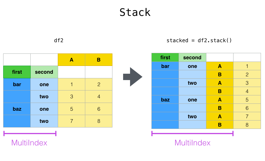
The stack() function “compresses” a level in the DataFrame columns to
produce either:
A
DataFrame, in the case of aMultiIndexin the columns.
If the columns have a MultiIndex, you can choose which level to stack. The
stacked level becomes the new lowest level in a MultiIndex on the columns:
In [25]: stacked = df2.stack()

In [26]: stacked
Out[26]:
first  second
bar    one     A    0.895717
               B    0.805244
       two     A   -1.206412
               B    2.565646
baz    one     A    1.431256
               B    1.340309
       two     A   -1.170299
               B   -0.226169
dtype: float64
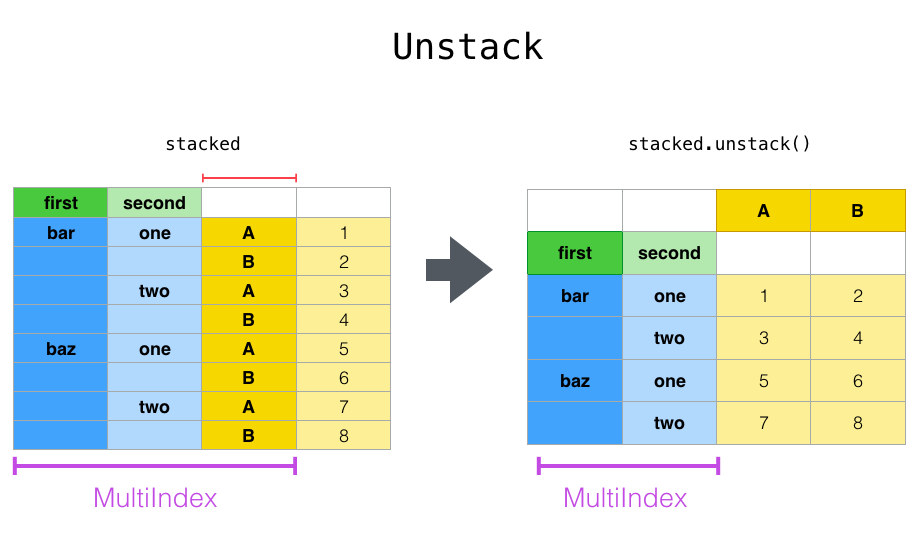
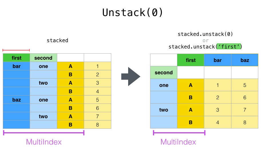
With a “stacked” DataFrame or Series (having a MultiIndex as the
index), the inverse operation of stack() is unstack(), which by default
unstacks the last level:
In [27]: stacked.unstack()
Out[27]:
                     A         B
first second
bar   one     0.895717  0.805244
      two    -1.206412  2.565646
baz   one     1.431256  1.340309
      two    -1.170299 -0.226169

In [28]: stacked.unstack(1)
Out[28]:
second        one       two
first
bar   A  0.895717 -1.206412
      B  0.805244  2.565646
baz   A  1.431256 -1.170299
      B  1.340309 -0.226169

In [29]: stacked.unstack(0)
Out[29]:
first          bar       baz
second
one    A  0.895717  1.431256
       B  0.805244  1.340309
two    A -1.206412 -1.170299
       B  2.565646 -0.226169
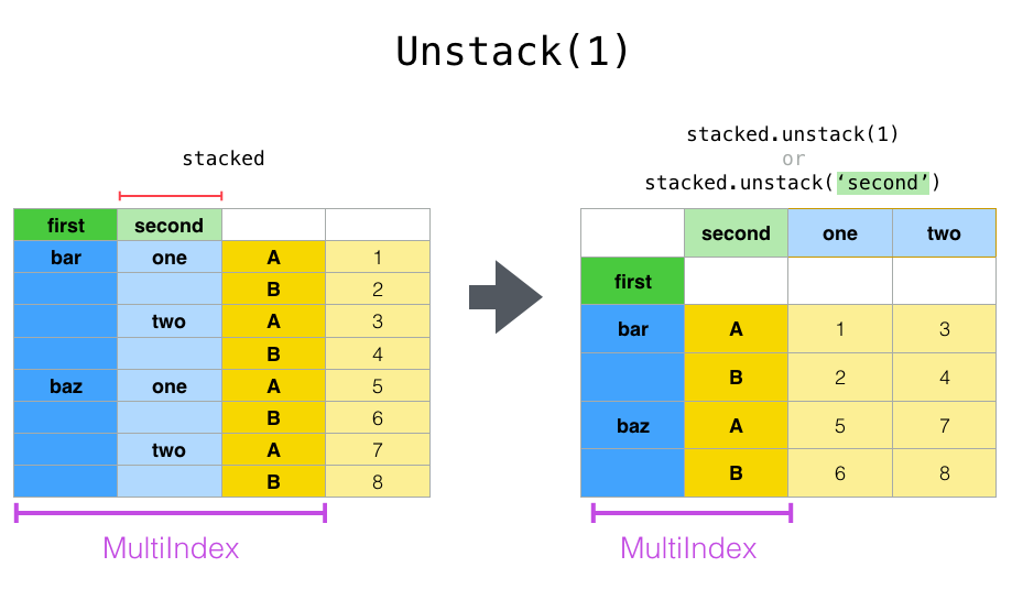
If the indexes have names, you can use the level names instead of specifying the level numbers:
In [30]: stacked.unstack("second")
Out[30]:
second        one       two
first
bar   A  0.895717 -1.206412
      B  0.805244  2.565646
baz   A  1.431256 -1.170299
      B  1.340309 -0.226169
Notice that the unstack() method implicitly sorts the index levels involved,
while stack() preserves the order of the stacked column level. Because
unstack() sorts, a call to stack() and then
unstack(), or vice versa, will result in a sorted copy of the original
DataFrame or Series. Here “sorted” is with respect to the order of the
MultiIndex.levels, which for a typical MultiIndex matches sorting by value:
In [31]: index = pd.MultiIndex.from_product([[2, 1], ["a", "b"]])

In [32]: df = pd.DataFrame(np.random.randn(4), index=index, columns=["A"])

In [33]: df
Out[33]:
            A
2 a -1.413681
  b  1.607920
1 a  1.024180
  b  0.569605

In [34]: all(df.unstack().stack() == df.sort_index())
Out[34]: True
Multiple levels#
You may also stack or unstack more than one level at a time by passing a list of levels, in which case the end result is as if each level in the list were processed individually.
In [35]: columns = pd.MultiIndex.from_tuples(
   ....:     [
   ....:         ("A", "cat", "long"),
   ....:         ("B", "cat", "long"),
   ....:         ("A", "dog", "short"),
   ....:         ("B", "dog", "short"),
   ....:     ],
   ....:     names=["exp", "animal", "hair_length"],
   ....: )
   ....:

In [36]: df = pd.DataFrame(np.random.randn(4, 4), columns=columns)

In [37]: df
Out[37]:
exp                 A         B         A         B
animal            cat       cat       dog       dog
hair_length      long      long     short     short
0            0.875906 -2.211372  0.974466 -2.006747
1           -0.410001 -0.078638  0.545952 -1.219217
2           -1.226825  0.769804 -1.281247 -0.727707
3           -0.121306 -0.097883  0.695775  0.341734

In [38]: df.stack(level=["animal", "hair_length"])
Out[38]:
exp                          A         B
  animal hair_length
0 cat    long         0.875906 -2.211372
  dog    short        0.974466 -2.006747
1 cat    long        -0.410001 -0.078638
  dog    short        0.545952 -1.219217
2 cat    long        -1.226825  0.769804
  dog    short       -1.281247 -0.727707
3 cat    long        -0.121306 -0.097883
  dog    short        0.695775  0.341734
The list of levels can contain either level names or level numbers but not a mixture of the two.
# df.stack(level=['animal', 'hair_length'])
# from above is equivalent to:
In [39]: df.stack(level=[1, 2])
Out[39]:
exp                          A         B
  animal hair_length
0 cat    long         0.875906 -2.211372
  dog    short        0.974466 -2.006747
1 cat    long        -0.410001 -0.078638
  dog    short        0.545952 -1.219217
2 cat    long        -1.226825  0.769804
  dog    short       -1.281247 -0.727707
3 cat    long        -0.121306 -0.097883
  dog    short        0.695775  0.341734
Missing data#
Unstacking can result in missing values if subgroups do not have the same set of labels. By default, missing values will be replaced with the default fill value for that data type.
In [40]: columns = pd.MultiIndex.from_tuples(
   ....:     [
   ....:         ("A", "cat"),
   ....:         ("B", "dog"),
   ....:         ("B", "cat"),
   ....:         ("A", "dog"),
   ....:     ],
   ....:     names=["exp", "animal"],
   ....: )
   ....:

In [41]: index = pd.MultiIndex.from_product(
   ....:     [("bar", "baz", "foo", "qux"), ("one", "two")], names=["first", "second"]
   ....: )
   ....:

In [42]: df = pd.DataFrame(np.random.randn(8, 4), index=index, columns=columns)

In [43]: df3 = df.iloc[[0, 1, 4, 7], [1, 2]]

In [44]: df3
Out[44]:
exp                  B
animal             dog       cat
first second
bar   one    -1.110336 -0.619976
      two     0.687738  0.176444
foo   one     1.314232  0.690579
qux   two     0.380396  0.084844

In [45]: df3.unstack()
Out[45]:
exp            B
animal       dog                 cat
second       one       two       one       two
first
bar    -1.110336  0.687738 -0.619976  0.176444
foo     1.314232       NaN  0.690579       NaN
qux          NaN  0.380396       NaN  0.084844
The missing value can be filled with a specific value with the fill_value argument.
In [46]: df3.unstack(fill_value=-1e9)
Out[46]:
exp                B
animal           dog                         cat
second           one           two           one           two
first
bar    -1.110336e+00  6.877384e-01 -6.199759e-01  1.764443e-01
foo     1.314232e+00 -1.000000e+09  6.905793e-01 -1.000000e+09
qux    -1.000000e+09  3.803956e-01 -1.000000e+09  8.484421e-02
melt() and wide_to_long()#
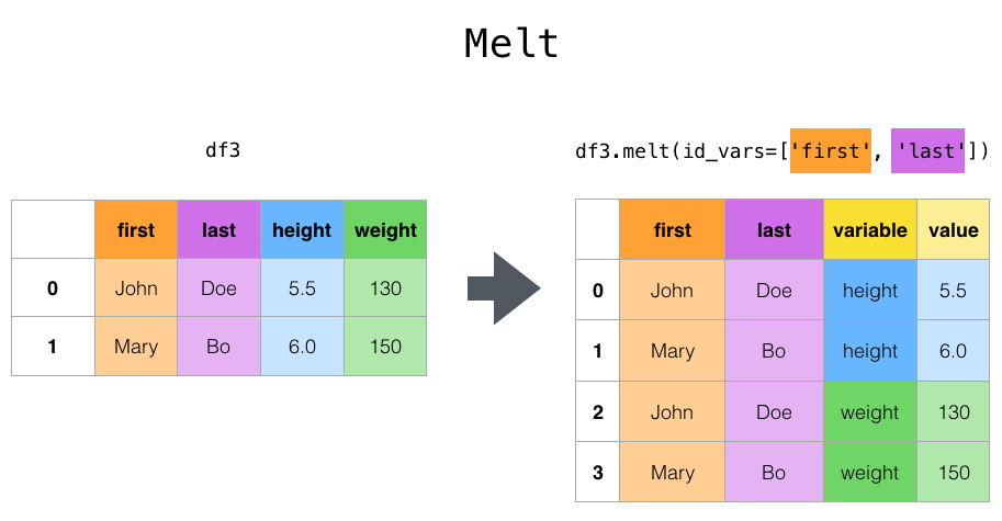
The top-level melt() function and the corresponding DataFrame.melt()
are useful to reshape a DataFrame into a format where one or more columns
are identifier variables, while all other columns, considered measured
variables, are “unpivoted” to the row axis, leaving just two non-identifier
columns, “variable” and “value”. The names of those columns can be customized
by supplying the var_name and value_name parameters.
In [47]: cheese = pd.DataFrame(
   ....:     {
   ....:         "first": ["John", "Mary"],
   ....:         "last": ["Doe", "Bo"],
   ....:         "height": [5.5, 6.0],
   ....:         "weight": [130, 150],
   ....:     }
   ....: )
   ....:

In [48]: cheese
Out[48]:
  first last  height  weight
0  John  Doe     5.5     130
1  Mary   Bo     6.0     150

In [49]: cheese.melt(id_vars=["first", "last"])
Out[49]:
  first last variable  value
0  John  Doe   height    5.5
1  Mary   Bo   height    6.0
2  John  Doe   weight  130.0
3  Mary   Bo   weight  150.0

In [50]: cheese.melt(id_vars=["first", "last"], var_name="quantity")
Out[50]:
  first last quantity  value
0  John  Doe   height    5.5
1  Mary   Bo   height    6.0
2  John  Doe   weight  130.0
3  Mary   Bo   weight  150.0
When transforming a DataFrame using melt(), the index will be ignored.
The original index values can be kept by setting the ignore_index parameter to False (default is True).
ignore_index=False will however duplicate index values.
In [51]: index = pd.MultiIndex.from_tuples([("person", "A"), ("person", "B")])

In [52]: cheese = pd.DataFrame(
   ....:     {
   ....:         "first": ["John", "Mary"],
   ....:         "last": ["Doe", "Bo"],
   ....:         "height": [5.5, 6.0],
   ....:         "weight": [130, 150],
   ....:     },
   ....:     index=index,
   ....: )
   ....:

In [53]: cheese
Out[53]:
         first last  height  weight
person A  John  Doe     5.5     130
       B  Mary   Bo     6.0     150

In [54]: cheese.melt(id_vars=["first", "last"])
Out[54]:
  first last variable  value
0  John  Doe   height    5.5
1  Mary   Bo   height    6.0
2  John  Doe   weight  130.0
3  Mary   Bo   weight  150.0

In [55]: cheese.melt(id_vars=["first", "last"], ignore_index=False)
Out[55]:
         first last variable  value
person A  John  Doe   height    5.5
       B  Mary   Bo   height    6.0
       A  John  Doe   weight  130.0
       B  Mary   Bo   weight  150.0
wide_to_long() is similar to melt() with more customization for
column matching.
In [56]: dft = pd.DataFrame(
   ....:     {
   ....:         "A1970": {0: "a", 1: "b", 2: "c"},
   ....:         "A1980": {0: "d", 1: "e", 2: "f"},
   ....:         "B1970": {0: 2.5, 1: 1.2, 2: 0.7},
   ....:         "B1980": {0: 3.2, 1: 1.3, 2: 0.1},
   ....:         "X": dict(zip(range(3), np.random.randn(3))),
   ....:     }
   ....: )
   ....:

In [57]: dft["id"] = dft.index

In [58]: dft
Out[58]:
  A1970 A1980  B1970  B1980         X  id
0     a     d    2.5    3.2  1.519970   0
1     b     e    1.2    1.3 -0.493662   1
2     c     f    0.7    0.1  0.600178   2

In [59]: pd.wide_to_long(dft, ["A", "B"], i="id", j="year")
Out[59]:
                X  A    B
id year
0  1970  1.519970  a  2.5
1  1970 -0.493662  b  1.2
2  1970  0.600178  c  0.7
0  1980  1.519970  d  3.2
1  1980 -0.493662  e  1.3
2  1980  0.600178  f  0.1
get_dummies() and from_dummies()#
To convert categorical variables of a Series into a “dummy” or “indicator”,
get_dummies() creates a new DataFrame with columns of the unique
variables and the values representing the presence of those variables per row.
In [60]: df = pd.DataFrame({"key": list("bbacab"), "data1": range(6)})

In [61]: pd.get_dummies(df["key"])
Out[61]:
       a      b      c
0  False   True  False
1  False   True  False
2   True  False  False
3  False  False   True
4   True  False  False
5  False   True  False

In [62]: df["key"].str.get_dummies()
Out[62]:
   a  b  c
0  0  1  0
1  0  1  0
2  1  0  0
3  0  0  1
4  1  0  0
5  0  1  0
prefix adds a prefix to the column names which is useful for merging the result
with the original DataFrame:
In [63]: dummies = pd.get_dummies(df["key"], prefix="key")

In [64]: dummies
Out[64]:
   key_a  key_b  key_c
0  False   True  False
1  False   True  False
2   True  False  False
3  False  False   True
4   True  False  False
5  False   True  False

In [65]: df[["data1"]].join(dummies)
Out[65]:
   data1  key_a  key_b  key_c
0      0  False   True  False
1      1  False   True  False
2      2   True  False  False
3      3  False  False   True
4      4   True  False  False
5      5  False   True  False
This function is often used along with discretization functions like cut():
In [66]: values = np.random.randn(10)

In [67]: values
Out[67]:
array([ 0.2742,  0.1329, -0.0237,  2.4102,  1.4505,  0.2061, -0.2519,
       -2.2136,  1.0633,  1.2661])

In [68]: bins = [0, 0.2, 0.4, 0.6, 0.8, 1]

In [69]: pd.get_dummies(pd.cut(values, bins))
Out[69]:
   (0.0, 0.2]  (0.2, 0.4]  (0.4, 0.6]  (0.6, 0.8]  (0.8, 1.0]
0       False        True       False       False       False
1        True       False       False       False       False
2       False       False       False       False       False
3       False       False       False       False       False
4       False       False       False       False       False
5       False        True       False       False       False
6       False       False       False       False       False
7       False       False       False       False       False
8       False       False       False       False       False
9       False       False       False       False       False
get_dummies() also accepts a DataFrame. By default, object, string,
or categorical type columns are encoded as dummy variables with other columns unaltered.
In [70]: df = pd.DataFrame({"A": ["a", "b", "a"], "B": ["c", "c", "b"], "C": [1, 2, 3]})

In [71]: pd.get_dummies(df)
Out[71]:
   C    A_a    A_b    B_b    B_c
0  1   True  False  False   True
1  2  False   True  False   True
2  3   True  False   True  False
Specifying the columns keyword will encode a column of any type.
In [72]: pd.get_dummies(df, columns=["A"])
Out[72]:
   B  C    A_a    A_b
0  c  1   True  False
1  c  2  False   True
2  b  3   True  False
As with the Series version, you can pass values for the prefix and
prefix_sep. By default the column name is used as the prefix and _ as
the prefix separator. You can specify prefix and prefix_sep in 3 ways:
string: Use the same value for
prefixorprefix_sepfor each column to be encoded.list: Must be the same length as the number of columns being encoded.
dict: Mapping column name to prefix.
In [73]: simple = pd.get_dummies(df, prefix="new_prefix")

In [74]: simple
Out[74]:
   C  new_prefix_a  new_prefix_b  new_prefix_b  new_prefix_c
0  1          True         False         False          True
1  2         False          True         False          True
2  3          True         False          True         False

In [75]: from_list = pd.get_dummies(df, prefix=["from_A", "from_B"])

In [76]: from_list
Out[76]:
   C  from_A_a  from_A_b  from_B_b  from_B_c
0  1      True     False     False      True
1  2     False      True     False      True
2  3      True     False      True     False

In [77]: from_dict = pd.get_dummies(df, prefix={"B": "from_B", "A": "from_A"})

In [78]: from_dict
Out[78]:
   C  from_A_a  from_A_b  from_B_b  from_B_c
0  1      True     False     False      True
1  2     False      True     False      True
2  3      True     False      True     False
To avoid collinearity when feeding the result to statistical models,
specify drop_first=True.
In [79]: s = pd.Series(list("abcaa"))

In [80]: pd.get_dummies(s)
Out[80]:
       a      b      c
0   True  False  False
1  False   True  False
2  False  False   True
3   True  False  False
4   True  False  False

In [81]: pd.get_dummies(s, drop_first=True)
Out[81]:
       b      c
0  False  False
1   True  False
2  False   True
3  False  False
4  False  False
When a column contains only one level, it will be omitted in the result.
In [82]: df = pd.DataFrame({"A": list("aaaaa"), "B": list("ababc")})

In [83]: pd.get_dummies(df)
Out[83]:
    A_a    B_a    B_b    B_c
0  True   True  False  False
1  True  False   True  False
2  True   True  False  False
3  True  False   True  False
4  True  False  False   True

In [84]: pd.get_dummies(df, drop_first=True)
Out[84]:
     B_b    B_c
0  False  False
1   True  False
2  False  False
3   True  False
4  False   True
The values can be cast to a different type using the dtype argument.
In [85]: df = pd.DataFrame({"A": list("abc"), "B": [1.1, 2.2, 3.3]})

In [86]: pd.get_dummies(df, dtype=np.float32).dtypes
Out[86]:
B      float64
A_a    float32
A_b    float32
A_c    float32
dtype: object
from_dummies() converts the output of get_dummies() back into
a Series of categorical values from indicator values.
In [87]: df = pd.DataFrame({"prefix_a": [0, 1, 0], "prefix_b": [1, 0, 1]})

In [88]: df
Out[88]:
   prefix_a  prefix_b
0         0         1
1         1         0
2         0         1

In [89]: pd.from_dummies(df, sep="_")
Out[89]:
  prefix
0      b
1      a
2      b
Dummy coded data only requires k - 1 categories to be included, in this case
the last category is the default category. The default category can be modified with
default_category.
In [90]: df = pd.DataFrame({"prefix_a": [0, 1, 0]})

In [91]: df
Out[91]:
   prefix_a
0         0
1         1
2         0

In [92]: pd.from_dummies(df, sep="_", default_category="b")
Out[92]:
  prefix
0      b
1      a
2      b
explode()#
For a DataFrame column with nested, list-like values, explode() will transform
each list-like value to a separate row. The resulting Index will be duplicated corresponding
to the index label from the original row:
In [93]: keys = ["panda1", "panda2", "panda3"]

In [94]: values = [["eats", "shoots"], ["shoots", "leaves"], ["eats", "leaves"]]

In [95]: df = pd.DataFrame({"keys": keys, "values": values})

In [96]: df
Out[96]:
     keys            values
0  panda1    [eats, shoots]
1  panda2  [shoots, leaves]
2  panda3    [eats, leaves]

In [97]: df["values"].explode()
Out[97]:
0      eats
0    shoots
1    shoots
1    leaves
2      eats
2    leaves
Name: values, dtype: str
DataFrame.explode can also explode the column in the DataFrame.
In [98]: df.explode("values")
Out[98]:
     keys  values
0  panda1    eats
0  panda1  shoots
1  panda2  shoots
1  panda2  leaves
2  panda3    eats
2  panda3  leaves
Series.explode() will replace empty lists with a missing value indicator and preserve scalar entries.
In [99]: s = pd.Series([[1, 2, 3], "foo", [], ["a", "b"]])

In [100]: s
Out[100]:
0    [1, 2, 3]
1          foo
2           []
3       [a, b]
dtype: object

In [101]: s.explode()
Out[101]:
0      1
0      2
0      3
1    foo
2    NaN
3      a
3      b
dtype: object
A comma-separated string value can be split into individual values in a list and then exploded to a new row.
In [102]: df = pd.DataFrame([{"var1": "a,b,c", "var2": 1}, {"var1": "d,e,f", "var2": 2}])

In [103]: df.assign(var1=df.var1.str.split(",")).explode("var1")
Out[103]:
  var1  var2
0    a     1
0    b     1
0    c     1
1    d     2
1    e     2
1    f     2
crosstab()#
Use crosstab() to compute a cross-tabulation of two (or more)
factors. By default crosstab() computes a frequency table of the factors
unless an array of values and an aggregation function are passed.
Any Series passed will have their name attributes used unless row or column
names for the cross-tabulation are specified
In [104]: a = np.array(["foo", "foo", "bar", "bar", "foo", "foo"], dtype=object)

In [105]: b = np.array(["one", "one", "two", "one", "two", "one"], dtype=object)

In [106]: c = np.array(["dull", "dull", "shiny", "dull", "dull", "shiny"], dtype=object)

In [107]: pd.crosstab(a, [b, c], rownames=["a"], colnames=["b", "c"])
Out[107]:
b    one        two
c   dull shiny dull shiny
a
bar    1     0    0     1
foo    2     1    1     0
If crosstab() receives only two Series, it will provide a frequency table.
In [108]: df = pd.DataFrame(
   .....:     {"A": [1, 2, 2, 2, 2], "B": [3, 3, 4, 4, 4], "C": [1, 1, np.nan, 1, 1]}
   .....: )
   .....:

In [109]: df
Out[109]:
   A  B    C
0  1  3  1.0
1  2  3  1.0
2  2  4  NaN
3  2  4  1.0
4  2  4  1.0

In [110]: pd.crosstab(df["A"], df["B"])
Out[110]:
B  3  4
A
1  1  0
2  1  3
crosstab() can also summarize to Categorical data.
In [111]: foo = pd.Categorical(["a", "b"], categories=["a", "b", "c"])

In [112]: bar = pd.Categorical(["d", "e"], categories=["d", "e", "f"])

In [113]: pd.crosstab(foo, bar)
Out[113]:
col_0  d  e
row_0
a      1  0
b      0  1
For Categorical data, to include all of data categories even if the actual data does
not contain any instances of a particular category, use dropna=False.
In [114]: pd.crosstab(foo, bar, dropna=False)
Out[114]:
col_0  d  e  f
row_0
a      1  0  0
b      0  1  0
c      0  0  0
Normalization#
Frequency tables can also be normalized to show percentages rather than counts
using the normalize argument:
In [115]: pd.crosstab(df["A"], df["B"], normalize=True)
Out[115]:
B    3    4
A
1  0.2  0.0
2  0.2  0.6
normalize can also normalize values within each row or within each column:
In [116]: pd.crosstab(df["A"], df["B"], normalize="columns")
Out[116]:
B    3    4
A
1  0.5  0.0
2  0.5  1.0
crosstab() can also accept a third Series and an aggregation function
(aggfunc) that will be applied to the values of the third Series within
each group defined by the first two Series:
In [117]: pd.crosstab(df["A"], df["B"], values=df["C"], aggfunc="sum")
Out[117]:
B    3    4
A
1  1.0  NaN
2  1.0  2.0
Adding margins#
margins=True will add a row and column with an All label with partial group aggregates
across the categories on the rows and columns:
In [118]: pd.crosstab(
   .....:     df["A"], df["B"], values=df["C"], aggfunc="sum", normalize=True, margins=True
   .....: )
   .....:
Out[118]:
B       3    4   All
A
1    0.25  0.0  0.25
2    0.25  0.5  0.75
All  0.50  0.5  1.00
cut()#
The cut() function computes groupings for the values of the input
array and is often used to transform continuous variables to discrete or
categorical variables:
An integer bins will form equal-width bins.
In [119]: ages = np.array([10, 15, 13, 12, 23, 25, 28, 59, 60])

In [120]: pd.cut(ages, bins=3)
Out[120]:
[(9.95, 26.667], (9.95, 26.667], (9.95, 26.667], (9.95, 26.667], (9.95, 26.667],
 (9.95, 26.667], (26.667, 43.333], (43.333, 60.0], (43.333, 60.0]]
Categories (3, interval[float64, right]): [(9.95, 26.667] < (26.667, 43.333] <
                                           (43.333, 60.0]]
A list of ordered bin edges will assign an interval for each variable.
In [121]: pd.cut(ages, bins=[0, 18, 35, 70])
Out[121]:
[(0, 18], (0, 18], (0, 18], (0, 18], (18, 35], (18, 35], (18, 35], (35, 70],
 (35, 70]]
Categories (3, interval[int64, right]): [(0, 18] < (18, 35] < (35, 70]]
If the bins keyword is an IntervalIndex, then these will be
used to bin the passed data.
In [122]: pd.cut(ages, bins=pd.IntervalIndex.from_breaks([0, 40, 70]))
Out[122]:
[(0, 40], (0, 40], (0, 40], (0, 40], (0, 40], (0, 40], (0, 40], (40, 70],
 (40, 70]]
Categories (2, interval[int64, right]): [(0, 40] < (40, 70]]
factorize()#
factorize() encodes 1 dimensional values into integer labels. Missing values
are encoded as -1.
In [123]: x = pd.Series(["A", "A", np.nan, "B", 3.14, np.inf])

In [124]: x
Out[124]:
0       A
1       A
2     NaN
3       B
4    3.14
5     inf
dtype: object

In [125]: labels, uniques = pd.factorize(x)

In [126]: labels
Out[126]: array([ 0,  0, -1,  1,  2,  3])

In [127]: uniques
Out[127]: Index(['A', 'B', 3.14, inf], dtype='object')
Categorical will similarly encode 1 dimensional values for further
categorical operations
In [128]: pd.Categorical(x)
Out[128]:
['A', 'A', NaN, 'B', 3.14, inf]
Categories (4, object): [3.14, inf, 'A', 'B']