

Indexing and selecting data#
The axis labeling information in pandas objects serves many purposes:
Identifies data (i.e. provides metadata) using known indicators, important for analysis, visualization, and interactive console display.
Enables automatic and explicit data alignment.
Allows intuitive getting and setting of subsets of the data set.
In this section, we will focus on the final point: namely, how to slice, dice, and generally get and set subsets of pandas objects. The primary focus will be on Series and DataFrame as they have received more development attention in this area.
Note
The Python and NumPy indexing operators [] and attribute operator .
provide quick and easy access to pandas data structures across a wide range
of use cases. This makes interactive work intuitive, as there’s little new
to learn if you already know how to deal with Python dictionaries and NumPy
arrays. However, since the type of the data to be accessed isn’t known in
advance, directly using standard operators has some optimization limits. For
production code, we recommended that you take advantage of the optimized
pandas data access methods exposed in this chapter.
See the MultiIndex / Advanced Indexing for MultiIndex and more advanced indexing documentation.
See the cookbook for some advanced strategies.
Different choices for indexing#
Object selection has had a number of user-requested additions in order to support more explicit location based indexing. pandas now supports three types of multi-axis indexing.
.locis primarily label based, but may also be used with a boolean array..locwill raiseKeyErrorwhen the items are not found. Allowed inputs are:A single label, e.g.
5or'a'(Note that5is interpreted as a label of the index. This use is not an integer position along the index.).A list or array of labels
['a', 'b', 'c'].A slice object with labels
'a':'f'(Note that contrary to usual Python slices, both the start and the stop are included, when present in the index! See Slicing with labels and Endpoints are inclusive.)A boolean array (any
NAvalues will be treated asFalse).A
callablefunction with one argument (the calling Series or DataFrame) and that returns valid output for indexing (one of the above).A tuple of row (and column) indices whose elements are one of the above inputs.
See more at Selection by Label.
.ilocis primarily integer position based (from0tolength-1of the axis), but may also be used with a boolean array..ilocwill raiseIndexErrorif a requested indexer is out-of-bounds, except slice indexers which allow out-of-bounds indexing. (this conforms with Python/NumPy slice semantics). Allowed inputs are:An integer e.g.
5.A list or array of integers
[4, 3, 0].A slice object with ints
1:7.A boolean array (any
NAvalues will be treated asFalse).A
callablefunction with one argument (the calling Series or DataFrame) and that returns valid output for indexing (one of the above).A tuple of row (and column) indices whose elements are one of the above inputs.
See more at Selection by Position, Advanced Indexing and Advanced Hierarchical.
.loc,.iloc, and also[]indexing can accept acallableas indexer. See more at Selection By Callable.Note
Destructuring tuple keys into row (and column) indexes occurs before callables are applied, so you cannot return a tuple from a callable to index both rows and columns.
Getting values from an object with multi-axes selection uses the following
notation (using .loc as an example, but the following applies to .iloc as
well). Any of the axes accessors may be the null slice :. Axes left out of
the specification are assumed to be :, e.g. p.loc['a'] is equivalent to
p.loc['a', :].
In [1]: ser = pd.Series(range(5), index=list("abcde"))

In [2]: ser.loc[["a", "c", "e"]]
Out[2]:
a    0
c    2
e    4
dtype: int64

In [3]: df = pd.DataFrame(np.arange(25).reshape(5, 5), index=list("abcde"), columns=list("abcde"))

In [4]: df.loc[["a", "c", "e"], ["b", "d"]]
Out[4]:
    b   d
a   1   3
c  11  13
e  21  23
Basics#
As mentioned when introducing the data structures in the last section, the primary function of indexing with [] (a.k.a. __getitem__
for those familiar with implementing class behavior in Python) is selecting out
lower-dimensional slices. The following table shows return type values when
indexing pandas objects with []:
Object Type |
Selection |
Return Value Type |
|---|---|---|
Series |
|
scalar value |
DataFrame |
|
|
DataFrame |
|
|
DataFrame |
|
|
The same principle applies to label-based selection with .loc: a
list-like of labels preserves the corresponding axis (so
df.loc[:, ["A"]] returns a DataFrame, even when the list contains a
single label), while a scalar label reduces the axis when labels on that
axis are unique (so df.loc[:, "A"] typically returns a Series; if
"A" is duplicated on the axis, a DataFrame is returned instead).
See Selection by label for details.
Here we construct a simple time series data set to use for illustrating the indexing functionality:
In [5]: dates = pd.date_range('1/1/2000', periods=8)

In [6]: df = pd.DataFrame(np.random.randn(8, 4),
   ...:                   index=dates, columns=['A', 'B', 'C', 'D'])
   ...:

In [7]: df
Out[7]:
                   A         B         C         D
2000-01-01  0.469112 -0.282863 -1.509059 -1.135632
2000-01-02  1.212112 -0.173215  0.119209 -1.044236
2000-01-03 -0.861849 -2.104569 -0.494929  1.071804
2000-01-04  0.721555 -0.706771 -1.039575  0.271860
2000-01-05 -0.424972  0.567020  0.276232 -1.087401
2000-01-06 -0.673690  0.113648 -1.478427  0.524988
2000-01-07  0.404705  0.577046 -1.715002 -1.039268
2000-01-08 -0.370647 -1.157892 -1.344312  0.844885
Note
None of the indexing functionality is time series specific unless specifically stated.
Thus, as per above, we have the most basic indexing using []:
In [8]: s = df['A']

In [9]: s[dates[5]]
Out[9]: np.float64(-0.6736897080883706)
You can pass a list of columns to [] to select columns in that order.
If a column is not contained in the DataFrame, an exception will be
raised. Multiple columns can also be set in this manner:
In [10]: df
Out[10]:
                   A         B         C         D
2000-01-01  0.469112 -0.282863 -1.509059 -1.135632
2000-01-02  1.212112 -0.173215  0.119209 -1.044236
2000-01-03 -0.861849 -2.104569 -0.494929  1.071804
2000-01-04  0.721555 -0.706771 -1.039575  0.271860
2000-01-05 -0.424972  0.567020  0.276232 -1.087401
2000-01-06 -0.673690  0.113648 -1.478427  0.524988
2000-01-07  0.404705  0.577046 -1.715002 -1.039268
2000-01-08 -0.370647 -1.157892 -1.344312  0.844885

In [11]: df[['B', 'A']] = df[['A', 'B']]

In [12]: df
Out[12]:
                   A         B         C         D
2000-01-01 -0.282863  0.469112 -1.509059 -1.135632
2000-01-02 -0.173215  1.212112  0.119209 -1.044236
2000-01-03 -2.104569 -0.861849 -0.494929  1.071804
2000-01-04 -0.706771  0.721555 -1.039575  0.271860
2000-01-05  0.567020 -0.424972  0.276232 -1.087401
2000-01-06  0.113648 -0.673690 -1.478427  0.524988
2000-01-07  0.577046  0.404705 -1.715002 -1.039268
2000-01-08 -1.157892 -0.370647 -1.344312  0.844885
You may find this useful for applying a transform (in-place) to a subset of the columns.
Warning
pandas aligns all AXES when setting Series and DataFrame from .loc.
This will not modify df because the column alignment is before value assignment.
In [13]: df[['A', 'B']]
Out[13]:
                   A         B
2000-01-01 -0.282863  0.469112
2000-01-02 -0.173215  1.212112
2000-01-03 -2.104569 -0.861849
2000-01-04 -0.706771  0.721555
2000-01-05  0.567020 -0.424972
2000-01-06  0.113648 -0.673690
2000-01-07  0.577046  0.404705
2000-01-08 -1.157892 -0.370647

In [14]: df.loc[:, ['B', 'A']] = df[['A', 'B']]

In [15]: df[['A', 'B']]
Out[15]:
                   A         B
2000-01-01 -0.282863  0.469112
2000-01-02 -0.173215  1.212112
2000-01-03 -2.104569 -0.861849
2000-01-04 -0.706771  0.721555
2000-01-05  0.567020 -0.424972
2000-01-06  0.113648 -0.673690
2000-01-07  0.577046  0.404705
2000-01-08 -1.157892 -0.370647
The correct way to swap column values is by using raw values:
In [16]: df.loc[:, ['B', 'A']] = df[['A', 'B']].to_numpy()

In [17]: df[['A', 'B']]
Out[17]:
                   A         B
2000-01-01  0.469112 -0.282863
2000-01-02  1.212112 -0.173215
2000-01-03 -0.861849 -2.104569
2000-01-04  0.721555 -0.706771
2000-01-05 -0.424972  0.567020
2000-01-06 -0.673690  0.113648
2000-01-07  0.404705  0.577046
2000-01-08 -0.370647 -1.157892
However, pandas does not align AXES when setting Series and DataFrame from .iloc
because .iloc operates by position.
This will modify df because the column alignment is not done before value assignment.
In [18]: df[['A', 'B']]
Out[18]:
                   A         B
2000-01-01  0.469112 -0.282863
2000-01-02  1.212112 -0.173215
2000-01-03 -0.861849 -2.104569
2000-01-04  0.721555 -0.706771
2000-01-05 -0.424972  0.567020
2000-01-06 -0.673690  0.113648
2000-01-07  0.404705  0.577046
2000-01-08 -0.370647 -1.157892

In [19]: df.iloc[:, [1, 0]] = df[['A', 'B']]

In [20]: df[['A','B']]
Out[20]:
                   A         B
2000-01-01 -0.282863  0.469112
2000-01-02 -0.173215  1.212112
2000-01-03 -2.104569 -0.861849
2000-01-04 -0.706771  0.721555
2000-01-05  0.567020 -0.424972
2000-01-06  0.113648 -0.673690
2000-01-07  0.577046  0.404705
2000-01-08 -1.157892 -0.370647
Attribute access#
You may access an index on a Series or column on a DataFrame directly
as an attribute:
In [21]: sa = pd.Series([1, 2, 3], index=list('abc'))

In [22]: dfa = df.copy()
In [23]: sa.b
Out[23]: np.int64(2)

In [24]: dfa.A
Out[24]:
2000-01-01   -0.282863
2000-01-02   -0.173215
2000-01-03   -2.104569
2000-01-04   -0.706771
2000-01-05    0.567020
2000-01-06    0.113648
2000-01-07    0.577046
2000-01-08   -1.157892
Freq: D, Name: A, dtype: float64
In [25]: sa.a = 5

In [26]: sa
Out[26]:
a    5
b    2
c    3
dtype: int64

In [27]: dfa.A = list(range(len(dfa.index)))  # ok if A already exists

In [28]: dfa
Out[28]:
            A         B         C         D
2000-01-01  0  0.469112 -1.509059 -1.135632
2000-01-02  1  1.212112  0.119209 -1.044236
2000-01-03  2 -0.861849 -0.494929  1.071804
2000-01-04  3  0.721555 -1.039575  0.271860
2000-01-05  4 -0.424972  0.276232 -1.087401
2000-01-06  5 -0.673690 -1.478427  0.524988
2000-01-07  6  0.404705 -1.715002 -1.039268
2000-01-08  7 -0.370647 -1.344312  0.844885

In [29]: dfa['A'] = list(range(len(dfa.index)))  # use this form to create a new column

In [30]: dfa
Out[30]:
            A         B         C         D
2000-01-01  0  0.469112 -1.509059 -1.135632
2000-01-02  1  1.212112  0.119209 -1.044236
2000-01-03  2 -0.861849 -0.494929  1.071804
2000-01-04  3  0.721555 -1.039575  0.271860
2000-01-05  4 -0.424972  0.276232 -1.087401
2000-01-06  5 -0.673690 -1.478427  0.524988
2000-01-07  6  0.404705 -1.715002 -1.039268
2000-01-08  7 -0.370647 -1.344312  0.844885
Warning
You can use this access only if the index element is a valid Python identifier, e.g.
s.1is not allowed. See here for an explanation of valid identifiers.The attribute will not be available if it conflicts with an existing method name, e.g.
s.minis not allowed, buts['min']is possible.Similarly, the attribute will not be available if it conflicts with any of the following list:
index,major_axis,minor_axis,items.In any of these cases, standard indexing will still work, e.g.
s['1'],s['min'], ands['index']will access the corresponding element or column.
If you are using the IPython environment, you may also use tab-completion to see these accessible attributes.
You can also assign a dict to a row of a DataFrame:
In [31]: x = pd.DataFrame({'x': [1, 2, 3], 'y': [3, 4, 5]})

In [32]: x.iloc[1] = {'x': 9, 'y': 99}

In [33]: x
Out[33]:
   x   y
0  1   3
1  9  99
2  3   5
You can use attribute access to modify an existing element of a Series or column of a DataFrame, but be careful;
if you try to use attribute access to create a new column, it creates a new attribute rather than a
new column and will this raise a UserWarning:
In [34]: df_new = pd.DataFrame({'one': [1., 2., 3.]})

In [35]: df_new.two = [4, 5, 6]

In [36]: df_new
Out[36]:
   one
0  1.0
1  2.0
2  3.0
Slicing ranges#
The most robust and consistent way of slicing ranges along arbitrary axes is
described in the Selection by Position section
detailing the .iloc method. For now, we explain the semantics of slicing using the [] operator.
Note
When the
Serieshas float indices, slicing will select by position.
With Series, the syntax works exactly as with an ndarray, returning a slice of the values and the corresponding labels:
In [37]: s[:5]
Out[37]:
2000-01-01    0.469112
2000-01-02    1.212112
2000-01-03   -0.861849
2000-01-04    0.721555
2000-01-05   -0.424972
Freq: D, Name: A, dtype: float64

In [38]: s[::2]
Out[38]:
2000-01-01    0.469112
2000-01-03   -0.861849
2000-01-05   -0.424972
2000-01-07    0.404705
Freq: 2D, Name: A, dtype: float64

In [39]: s[::-1]
Out[39]:
2000-01-08   -0.370647
2000-01-07    0.404705
2000-01-06   -0.673690
2000-01-05   -0.424972
2000-01-04    0.721555
2000-01-03   -0.861849
2000-01-02    1.212112
2000-01-01    0.469112
Freq: -1D, Name: A, dtype: float64
Note that setting works as well:
In [40]: s2 = s.copy()

In [41]: s2[:5] = 0

In [42]: s2
Out[42]:
2000-01-01    0.000000
2000-01-02    0.000000
2000-01-03    0.000000
2000-01-04    0.000000
2000-01-05    0.000000
2000-01-06   -0.673690
2000-01-07    0.404705
2000-01-08   -0.370647
Freq: D, Name: A, dtype: float64
With DataFrame, slicing inside of [] slices the rows. This is provided
largely as a convenience since it is such a common operation.
In [43]: df[:3]
Out[43]:
                   A         B         C         D
2000-01-01 -0.282863  0.469112 -1.509059 -1.135632
2000-01-02 -0.173215  1.212112  0.119209 -1.044236
2000-01-03 -2.104569 -0.861849 -0.494929  1.071804

In [44]: df[::-1]
Out[44]:
                   A         B         C         D
2000-01-08 -1.157892 -0.370647 -1.344312  0.844885
2000-01-07  0.577046  0.404705 -1.715002 -1.039268
2000-01-06  0.113648 -0.673690 -1.478427  0.524988
2000-01-05  0.567020 -0.424972  0.276232 -1.087401
2000-01-04 -0.706771  0.721555 -1.039575  0.271860
2000-01-03 -2.104569 -0.861849 -0.494929  1.071804
2000-01-02 -0.173215  1.212112  0.119209 -1.044236
2000-01-01 -0.282863  0.469112 -1.509059 -1.135632
Selection by label#
Warning
.locis strict when you present slicers that are not compatible (or convertible) with the index type. For example using integers in aDatetimeIndex. These will raise aTypeError.In [45]: dfl = pd.DataFrame(np.random.randn(5, 4), ....: columns=list('ABCD'), ....: index=pd.date_range('20130101', periods=5)) ....: In [46]: dfl Out[46]: A B C D 2013-01-01 1.075770 -0.109050 1.643563 -1.469388 2013-01-02 0.357021 -0.674600 -1.776904 -0.968914 2013-01-03 -1.294524 0.413738 0.276662 -0.472035 2013-01-04 -0.013960 -0.362543 -0.006154 -0.923061 2013-01-05 0.895717 0.805244 -1.206412 2.565646 In [47]: dfl.loc[2:3] --------------------------------------------------------------------------- TypeError Traceback (most recent call last) Cell In[47], line 1 ----> 1 dfl.loc[2:3] File ~/work/pandas/pandas/pandas/core/indexing.py:1287, in _LocationIndexer.__getitem__(self, key) 1285 maybe_callable = com.apply_if_callable(key, self.obj) 1286 maybe_callable = self._raise_callable_usage(key, maybe_callable) -> 1287 return self._getitem_axis(maybe_callable, axis=axis) File ~/work/pandas/pandas/pandas/core/indexing.py:1859, in _LocIndexer._getitem_axis(self, key, axis) 1857 if isinstance(key, slice): 1858 self._validate_key(key, axis) -> 1859 return self._get_slice_axis(key, axis=axis) 1860 elif com.is_bool_indexer(key): 1861 return self._getbool_axis(key, axis=axis) File ~/work/pandas/pandas/pandas/core/indexing.py:1923, in _LocIndexer._get_slice_axis(self, slice_obj, axis) 1920 return obj.copy(deep=False) 1922 labels = obj._get_axis(axis) -> 1923 indexer = labels.slice_indexer(slice_obj.start, slice_obj.stop, slice_obj.step) 1925 if isinstance(indexer, slice): 1926 return self.obj._slice(indexer, axis=axis) File ~/work/pandas/pandas/pandas/core/indexes/datetimes.py:1298, in DatetimeIndex.slice_indexer(self, start, end, step) 1290 # GH#33146 if start and end are combinations of str and None and Index is not 1291 # monotonic, we can not use Index.slice_indexer because it does not honor the 1292 # actual elements, is only searching for start and end 1293 if ( 1294 check_str_or_none(start) 1295 or check_str_or_none(end) 1296 or self.is_monotonic_increasing 1297 ): -> 1298 return Index.slice_indexer(self, start, end, step) 1300 mask = np.array(True) 1301 in_index = True File ~/work/pandas/pandas/pandas/core/indexes/base.py:7042, in Index.slice_indexer(self, start, end, step) 6991 def slice_indexer( 6992 self, 6993 start: Hashable | None = None, 6994 end: Hashable | None = None, 6995 step: int | None = None, 6996 ) -> slice: 6997 """ 6998 Compute the slice indexer for input labels and step. 6999 (...) 7040 slice(1, 3, None) 7041 """ -> 7042 start_slice, end_slice = self.slice_locs(start, end, step=step) 7044 # return a slice 7045 if not is_scalar(start_slice): File ~/work/pandas/pandas/pandas/core/indexes/base.py:7319, in Index.slice_locs(self, start, end, step) 7317 start_slice = None 7318 if start is not None: -> 7319 start_slice = self.get_slice_bound(start, "left") 7320 if start_slice is None: 7321 start_slice = 0 File ~/work/pandas/pandas/pandas/core/indexes/base.py:7205, in Index.get_slice_bound(self, label, side) 7201 original_label = label 7203 # For datetime indices label may be a string that has to be converted 7204 # to datetime boundary according to its resolution. -> 7205 label = self._maybe_cast_slice_bound(label, side) 7207 # we need to look up the label 7208 try: File ~/work/pandas/pandas/pandas/core/indexes/datetimes.py:1258, in DatetimeIndex._maybe_cast_slice_bound(self, label, side) 1249 label = Timestamp(label).to_pydatetime() 1250 warnings.warn( 1251 # GH#35830 deprecate last remaining inconsistent date treatment 1252 "Slicing with a datetime.date object is deprecated. " (...) 1255 stacklevel=find_stack_level(), 1256 ) -> 1258 label = super()._maybe_cast_slice_bound(label, side) 1259 self._data._assert_tzawareness_compat(label) 1260 return Timestamp(label) File ~/work/pandas/pandas/pandas/core/indexes/datetimelike.py:617, in DatetimeIndexOpsMixin._maybe_cast_slice_bound(self, label, side) 615 return lower if side == "left" else upper 616 elif not isinstance(label, self._data._recognized_scalars): --> 617 self._raise_invalid_indexer("slice", label) 619 return label File ~/work/pandas/pandas/pandas/core/indexes/base.py:4277, in Index._raise_invalid_indexer(self, form, key, reraise) 4275 if reraise is not lib.no_default: 4276 raise TypeError(msg) from reraise -> 4277 raise TypeError(msg) TypeError: cannot do slice indexing on DatetimeIndex with these indexers [2] of type int
String likes in slicing can be convertible to the type of the index and lead to natural slicing.
In [48]: dfl.loc['20130102':'20130104']
Out[48]:
                   A         B         C         D
2013-01-02  0.357021 -0.674600 -1.776904 -0.968914
2013-01-03 -1.294524  0.413738  0.276662 -0.472035
2013-01-04 -0.013960 -0.362543 -0.006154 -0.923061
pandas provides a suite of methods in order to have purely label based indexing. This is a strict inclusion based protocol.
Every label asked for must be in the index, or a KeyError will be raised.
When slicing, both the start bound AND the stop bound are included, if present in the index.
Integers are valid labels, but they refer to the label and not the position.
The .loc attribute is the primary access method. The following are valid inputs:
A single label, e.g.
5or'a'(Note that5is interpreted as a label of the index. This use is not an integer position along the index.).A list or array of labels
['a', 'b', 'c'].A slice object with labels
'a':'f'. Note that contrary to usual Python slices, both the start and the stop are included, when present in the index! See Slicing with labels.A boolean array.
A
callable, see Selection By Callable.
In [49]: s1 = pd.Series(np.random.randn(6), index=list('abcdef'))

In [50]: s1
Out[50]:
a    1.431256
b    1.340309
c   -1.170299
d   -0.226169
e    0.410835
f    0.813850
dtype: float64

In [51]: s1.loc['c':]
Out[51]:
c   -1.170299
d   -0.226169
e    0.410835
f    0.813850
dtype: float64

In [52]: s1.loc['b']
Out[52]: np.float64(1.3403088497993827)
Note that setting works as well:
In [53]: s1.loc['c':] = 0

In [54]: s1
Out[54]:
a    1.431256
b    1.340309
c    0.000000
d    0.000000
e    0.000000
f    0.000000
dtype: float64
With a DataFrame:
In [55]: df1 = pd.DataFrame(np.random.randn(6, 4),
   ....:                    index=list('abcdef'),
   ....:                    columns=list('ABCD'))
   ....:

In [56]: df1
Out[56]:
          A         B         C         D
a  0.132003 -0.827317 -0.076467 -1.187678
b  1.130127 -1.436737 -1.413681  1.607920
c  1.024180  0.569605  0.875906 -2.211372
d  0.974466 -2.006747 -0.410001 -0.078638
e  0.545952 -1.219217 -1.226825  0.769804
f -1.281247 -0.727707 -0.121306 -0.097883

In [57]: df1.loc[['a', 'b', 'd'], :]
Out[57]:
          A         B         C         D
a  0.132003 -0.827317 -0.076467 -1.187678
b  1.130127 -1.436737 -1.413681  1.607920
d  0.974466 -2.006747 -0.410001 -0.078638
Accessing via label slices:
In [58]: df1.loc['d':, 'A':'C']
Out[58]:
          A         B         C
d  0.974466 -2.006747 -0.410001
e  0.545952 -1.219217 -1.226825
f -1.281247 -0.727707 -0.121306
For getting a cross section using a label (equivalent to df.xs('a')):
In [59]: df1.loc['a']
Out[59]:
A    0.132003
B   -0.827317
C   -0.076467
D   -1.187678
Name: a, dtype: float64
For getting values with a boolean array:
In [60]: df1.loc['a'] > 0
Out[60]:
A     True
B    False
C    False
D    False
Name: a, dtype: bool

In [61]: df1.loc[:, df1.loc['a'] > 0]
Out[61]:
          A
a  0.132003
b  1.130127
c  1.024180
d  0.974466
e  0.545952
f -1.281247
NA values in a boolean array propagate as False:
In [62]: mask = pd.array([True, False, True, False, pd.NA, False], dtype="boolean")

In [63]: mask
Out[63]:
<BooleanArray>
[True, False, True, False, <NA>, False]
Length: 6, dtype: boolean

In [64]: df1[mask]
Out[64]:
          A         B         C         D
a  0.132003 -0.827317 -0.076467 -1.187678
c  1.024180  0.569605  0.875906 -2.211372
For getting a value explicitly:
# this is also equivalent to ``df1.at['a','A']``
In [65]: df1.loc['a', 'A']
Out[65]: np.float64(0.13200317033032932)
Slicing with labels#
When using .loc with slices, if both the start and the stop labels are
present in the index, then elements located between the two (including them)
are returned:
In [66]: s = pd.Series(list('abcde'), index=[0, 3, 2, 5, 4])

In [67]: s.loc[3:5]
Out[67]:
3    b
2    c
5    d
dtype: str
If the index is sorted, and can be compared against start and stop labels, then slicing will still work as expected, by selecting labels which rank between the two:
In [68]: s.sort_index()
Out[68]:
0    a
2    c
3    b
4    e
5    d
dtype: str

In [69]: s.sort_index().loc[1:6]
Out[69]:
2    c
3    b
4    e
5    d
dtype: str
However, if at least one of the two is absent and the index is not sorted, an
error will be raised (since doing otherwise would be computationally expensive,
as well as potentially ambiguous for mixed type indexes). For instance, in the
above example, s.loc[1:6] would raise KeyError.
For the rationale behind this behavior, see Endpoints are inclusive.
In [70]: s = pd.Series(list('abcdef'), index=[0, 3, 2, 5, 4, 2])

In [71]: s.loc[3:5]
Out[71]:
3    b
2    c
5    d
dtype: str
Also, if the index has duplicate labels and either the start or the stop label is duplicated,
an error will be raised. For instance, in the above example, s.loc[2:5] would raise a KeyError.
For more information about duplicate labels, see Duplicate Labels.
When using a slice with a step, such as .loc[start:stop:step], note that
start and stop are interpreted as labels, while step is applied over
the positional index within that label range. This means a stepped slice
will behave differently than using the labels range(start, stop, step) when
the index is not contiguous integers.
For example, in a Series with a non-contiguous integer index:
In [72]: s = pd.Series(range(10), index=[0, 5, 10, 15, 20, 25, 30, 35, 40, 45])

In [73]: s.loc[10:50:5]              # (10), then skip 5 positions → 35 only
Out[73]:
10    2
35    7
dtype: int64

In [74]: s.loc[[10, 15, 20, 25]]     # explicit label selection
Out[74]:
10    2
15    3
20    4
25    5
dtype: int64
The first applies step across positional locations between the start/stop labels. The second selects each label directly.
Similarly, with a string-based index, the behavior is identical:
In [75]: s = pd.Series(range(10), index=['a', 'b', 'c', 'd', 'e', 'f', 'g', 'h', 'i', 'j'])

In [76]: s.loc['b':'i':2]            # Start at 'b' (position 1), stop at 'i' (position 8), step 2 positions → 'b', 'd', 'f', 'h'
Out[76]:
b    1
d    3
f    5
h    7
dtype: int64

In [77]: s.loc[['b', 'd', 'f', 'h']] # explicit label selection
Out[77]:
b    1
d    3
f    5
h    7
dtype: int64
In both cases, start and stop determine the label boundaries (inclusive), while step skips positions within that range, regardless of the index type.
Selection by position#
pandas provides a suite of methods in order to get purely integer based indexing. The semantics follow closely Python and NumPy slicing. These are 0-based indexing. When slicing, the start bound is included, while the upper bound is excluded. Trying to use a non-integer, even a valid label will raise an IndexError.
The .iloc attribute is the primary access method. The following are valid inputs:
An integer e.g.
5.A list or array of integers
[4, 3, 0].A slice object with ints
1:7.A boolean array.
A
callable, see Selection By Callable.A tuple of row (and column) indexes, whose elements are one of the above types.
In [78]: s1 = pd.Series(np.random.randn(5), index=list(range(0, 10, 2)))

In [79]: s1
Out[79]:
0    0.695775
2    0.341734
4    0.959726
6   -1.110336
8   -0.619976
dtype: float64

In [80]: s1.iloc[:3]
Out[80]:
0    0.695775
2    0.341734
4    0.959726
dtype: float64

In [81]: s1.iloc[3]
Out[81]: np.float64(-1.110336102891167)
Note that setting works as well:
In [82]: s1.iloc[:3] = 0

In [83]: s1
Out[83]:
0    0.000000
2    0.000000
4    0.000000
6   -1.110336
8   -0.619976
dtype: float64
With a DataFrame:
In [84]: df1 = pd.DataFrame(np.random.randn(6, 4),
   ....:                    index=list(range(0, 12, 2)),
   ....:                    columns=list(range(0, 8, 2)))
   ....:

In [85]: df1
Out[85]:
           0         2         4         6
0   0.149748 -0.732339  0.687738  0.176444
2   0.403310 -0.154951  0.301624 -2.179861
4  -1.369849 -0.954208  1.462696 -1.743161
6  -0.826591 -0.345352  1.314232  0.690579
8   0.995761  2.396780  0.014871  3.357427
10 -0.317441 -1.236269  0.896171 -0.487602
Select via integer slicing:
In [86]: df1.iloc[:3]
Out[86]:
          0         2         4         6
0  0.149748 -0.732339  0.687738  0.176444
2  0.403310 -0.154951  0.301624 -2.179861
4 -1.369849 -0.954208  1.462696 -1.743161

In [87]: df1.iloc[1:5, 2:4]
Out[87]:
          4         6
2  0.301624 -2.179861
4  1.462696 -1.743161
6  1.314232  0.690579
8  0.014871  3.357427
Select via integer list:
In [88]: df1.iloc[[1, 3, 5], [1, 3]]
Out[88]:
           2         6
2  -0.154951 -2.179861
6  -0.345352  0.690579
10 -1.236269 -0.487602
In [89]: df1.iloc[1:3, :]
Out[89]:
          0         2         4         6
2  0.403310 -0.154951  0.301624 -2.179861
4 -1.369849 -0.954208  1.462696 -1.743161
In [90]: df1.iloc[:, 1:3]
Out[90]:
           2         4
0  -0.732339  0.687738
2  -0.154951  0.301624
4  -0.954208  1.462696
6  -0.345352  1.314232
8   2.396780  0.014871
10 -1.236269  0.896171
# this is also equivalent to ``df1.iat[1,1]``
In [91]: df1.iloc[1, 1]
Out[91]: np.float64(-0.1549507744249032)
For getting a cross section using an integer position (equiv to df.xs(1)):
In [92]: df1.iloc[1]
Out[92]:
0    0.403310
2   -0.154951
4    0.301624
6   -2.179861
Name: 2, dtype: float64
Out of range slice indexes are handled gracefully just as in Python/NumPy.
# these are allowed in Python/NumPy.
In [93]: x = list('abcdef')

In [94]: x
Out[94]: ['a', 'b', 'c', 'd', 'e', 'f']

In [95]: x[4:10]
Out[95]: ['e', 'f']

In [96]: x[8:10]
Out[96]: []

In [97]: s = pd.Series(x)

In [98]: s
Out[98]:
0    a
1    b
2    c
3    d
4    e
5    f
dtype: str

In [99]: s.iloc[4:10]
Out[99]:
4    e
5    f
dtype: str

In [100]: s.iloc[8:10]
Out[100]: Series([], dtype: str)
Note that using slices that go out of bounds can result in an empty axis (e.g. an empty DataFrame being returned).
In [101]: dfl = pd.DataFrame(np.random.randn(5, 2), columns=list('AB'))

In [102]: dfl
Out[102]:
          A         B
0 -0.082240 -2.182937
1  0.380396  0.084844
2  0.432390  1.519970
3 -0.493662  0.600178
4  0.274230  0.132885

In [103]: dfl.iloc[:, 2:3]
Out[103]:
Empty DataFrame
Columns: []
Index: [0, 1, 2, 3, 4]

In [104]: dfl.iloc[:, 1:3]
Out[104]:
          B
0 -2.182937
1  0.084844
2  1.519970
3  0.600178
4  0.132885

In [105]: dfl.iloc[4:6]
Out[105]:
         A         B
4  0.27423  0.132885
A single indexer that is out of bounds will raise an IndexError.
A list of indexers where any element is out of bounds will raise an
IndexError.
In [106]: dfl.iloc[[4, 5, 6]]
---------------------------------------------------------------------------
IndexError                                Traceback (most recent call last)
File ~/work/pandas/pandas/pandas/core/indexing.py:2339, in _iLocIndexer._get_list_axis(self, key, axis)
   2338 try:
-> 2339     return self.obj.take(key, axis=axis)
   2340 except IndexError as err:
   2341     # re-raise with different error message, e.g. test_getitem_ndarray_3d

File ~/work/pandas/pandas/pandas/core/generic.py:4193, in NDFrame.take(self, indices, axis, **kwargs)
   4191             return self.copy(deep=False)
   4192
-> 4193         new_data = self._mgr.take(
   4194             indices,

File ~/work/pandas/pandas/pandas/core/internals/managers.py:1086, in BaseBlockManager.take(self, indexer, axis, verify)
   1085 n = self.shape[axis]
-> 1086 indexer = maybe_convert_indices(indexer, n, verify=verify)
   1088 new_labels = self.axes[axis].take(indexer)

File ~/work/pandas/pandas/pandas/core/indexers/utils.py:284, in maybe_convert_indices(indices, n, verify)
    283     if mask.any():
--> 284         raise IndexError("indices are out-of-bounds")
    285 return indices

IndexError: indices are out-of-bounds

The above exception was the direct cause of the following exception:

IndexError                                Traceback (most recent call last)
Cell In[106], line 1
----> 1 dfl.iloc[[4, 5, 6]]

File ~/work/pandas/pandas/pandas/core/indexing.py:1287, in _LocationIndexer.__getitem__(self, key)
   1285 maybe_callable = com.apply_if_callable(key, self.obj)
   1286 maybe_callable = self._raise_callable_usage(key, maybe_callable)
-> 1287 return self._getitem_axis(maybe_callable, axis=axis)

File ~/work/pandas/pandas/pandas/core/indexing.py:2368, in _iLocIndexer._getitem_axis(self, key, axis)
   2366 # a list of integers
   2367 elif is_list_like_indexer(key):
-> 2368     return self._get_list_axis(key, axis=axis)
   2370 # a single integer
   2371 else:
   2372     key = item_from_zerodim(key)

File ~/work/pandas/pandas/pandas/core/indexing.py:2342, in _iLocIndexer._get_list_axis(self, key, axis)
   2339     return self.obj.take(key, axis=axis)
   2340 except IndexError as err:
   2341     # re-raise with different error message, e.g. test_getitem_ndarray_3d
-> 2342     raise IndexError("positional indexers are out-of-bounds") from err

IndexError: positional indexers are out-of-bounds
In [107]: dfl.iloc[:, 4]
---------------------------------------------------------------------------
IndexError                                Traceback (most recent call last)
Cell In[107], line 1
----> 1 dfl.iloc[:, 4]

File ~/work/pandas/pandas/pandas/core/indexing.py:1280, in _LocationIndexer.__getitem__(self, key)
   1278     if self._is_scalar_access(key):
   1279         return self.obj._get_value(*key, takeable=self._takeable)
-> 1280     return self._getitem_tuple(key)
   1281 else:
   1282     # we by definition only have the 0th axis
   1283     axis = self.axis or 0

File ~/work/pandas/pandas/pandas/core/indexing.py:2315, in _iLocIndexer._getitem_tuple(self, tup)
   2314 def _getitem_tuple(self, tup: tuple):
-> 2315     tup = self._validate_tuple_indexer(tup)
   2316     with suppress(IndexingError):
   2317         return self._getitem_lowerdim(tup)

File ~/work/pandas/pandas/pandas/core/indexing.py:1069, in _LocationIndexer._validate_tuple_indexer(self, key)
   1067 for i, k in enumerate(key):
   1068     try:
-> 1069         self._validate_key(k, i)
   1070     except ValueError as err:
   1071         raise ValueError(
   1072             f"Location based indexing can only have [{self._valid_types}] types"
   1073         ) from err

File ~/work/pandas/pandas/pandas/core/indexing.py:2209, in _iLocIndexer._validate_key(self, key, axis)
   2207     return
   2208 elif is_integer(key):
-> 2209     self._validate_integer(key, axis)
   2210 elif isinstance(key, tuple):
   2211     # a tuple should already have been caught by this point
   2212     # so don't treat a tuple as a valid indexer
   2213     raise IndexingError("Too many indexers")

File ~/work/pandas/pandas/pandas/core/indexing.py:2310, in _iLocIndexer._validate_integer(self, key, axis)
   2308 len_axis = len(self.obj._get_axis(axis))
   2309 if key >= len_axis or key < -len_axis:
-> 2310     raise IndexError("single positional indexer is out-of-bounds")

IndexError: single positional indexer is out-of-bounds
Selection by callable#
.loc, .iloc, and also [] indexing can accept a callable as indexer.
The callable must be a function with one argument (the calling Series or DataFrame) that returns valid output for indexing.
Note
For .iloc indexing, returning a tuple from the callable is
not supported, since tuple destructuring for row and column indexes
occurs before applying callables.
In [108]: df1 = pd.DataFrame(np.random.randn(6, 4),
   .....:                    index=list('abcdef'),
   .....:                    columns=list('ABCD'))
   .....:

In [109]: df1
Out[109]:
          A         B         C         D
a -0.023688  2.410179  1.450520  0.206053
b -0.251905 -2.213588  1.063327  1.266143
c  0.299368 -0.863838  0.408204 -1.048089
d -0.025747 -0.988387  0.094055  1.262731
e  1.289997  0.082423 -0.055758  0.536580
f -0.489682  0.369374 -0.034571 -2.484478

In [110]: df1.loc[lambda df: df['A'] > 0, :]
Out[110]:
          A         B         C         D
c  0.299368 -0.863838  0.408204 -1.048089
e  1.289997  0.082423 -0.055758  0.536580

In [111]: df1.loc[:, lambda df: ['A', 'B']]
Out[111]:
          A         B
a -0.023688  2.410179
b -0.251905 -2.213588
c  0.299368 -0.863838
d -0.025747 -0.988387
e  1.289997  0.082423
f -0.489682  0.369374

In [112]: df1.iloc[:, lambda df: [0, 1]]
Out[112]:
          A         B
a -0.023688  2.410179
b -0.251905 -2.213588
c  0.299368 -0.863838
d -0.025747 -0.988387
e  1.289997  0.082423
f -0.489682  0.369374

In [113]: df1[lambda df: df.columns[0]]
Out[113]:
a   -0.023688
b   -0.251905
c    0.299368
d   -0.025747
e    1.289997
f   -0.489682
Name: A, dtype: float64
You can use callable indexing in Series.
In [114]: df1['A'].loc[lambda s: s > 0]
Out[114]:
c    0.299368
e    1.289997
Name: A, dtype: float64
Using these methods / indexers, you can chain data selection operations without using a temporary variable.
In [115]: bb = pd.read_csv('data/baseball.csv', index_col='id')

In [116]: (bb.groupby(['year', 'team']).sum(numeric_only=True)
   .....:    .loc[lambda df: df['r'] > 100])
   .....:
Out[116]:
           stint    g    ab    r    h  ...   ibb   hbp    sh    sf  gidp
year team                              ...
2007 CIN       6  379   745  101  203  ...  14.0   1.0   1.0  15.0  18.0
     DET       5  301  1062  162  283  ...   3.0  10.0   4.0   8.0  28.0
     HOU       4  311   926  109  218  ...   3.0   9.0  16.0   6.0  17.0
     LAN      11  413  1021  153  293  ...   8.0   9.0   3.0   8.0  29.0
     NYN      13  622  1854  240  509  ...  24.0  23.0  18.0  15.0  48.0
     SFN       5  482  1305  198  337  ...  51.0   8.0  16.0   6.0  41.0
     TEX       2  198   729  115  200  ...   4.0   5.0   2.0   8.0  16.0
     TOR       4  459  1408  187  378  ...  16.0  12.0   4.0  16.0  38.0

[8 rows x 18 columns]
Combining positional and label-based indexing#
If you wish to get the 0th and the 2nd elements from the index in the ‘A’ column, you can do:
In [117]: dfd = pd.DataFrame({'A': [1, 2, 3],
   .....:                     'B': [4, 5, 6]},
   .....:                    index=list('abc'))
   .....:

In [118]: dfd
Out[118]:
   A  B
a  1  4
b  2  5
c  3  6

In [119]: dfd.loc[dfd.index[[0, 2]], 'A']
Out[119]:
a    1
c    3
Name: A, dtype: int64
This can also be expressed using .iloc, by explicitly getting locations on the indexers, and using
positional indexing to select things.
In [120]: dfd.iloc[[0, 2], dfd.columns.get_loc('A')]
Out[120]:
a    1
c    3
Name: A, dtype: int64
For getting multiple indexers, using .get_indexer:
In [121]: dfd.iloc[[0, 2], dfd.columns.get_indexer(['A', 'B'])]
Out[121]:
   A  B
a  1  4
c  3  6
Reindexing#
The idiomatic way to achieve selecting potentially not-found elements is via .reindex(). See also the section on reindexing.
In [122]: s = pd.Series([1, 2, 3])

In [123]: s.reindex([1, 2, 3])
Out[123]:
1    2.0
2    3.0
3    NaN
dtype: float64
Alternatively, if you want to select only valid keys, the following is idiomatic and efficient; it is guaranteed to preserve the dtype of the selection.
In [124]: labels = [1, 2, 3]

In [125]: s.loc[s.index.intersection(labels)]
Out[125]:
1    2
2    3
dtype: int64
Having a duplicated index will raise for a .reindex():
In [126]: s = pd.Series(np.arange(4), index=['a', 'a', 'b', 'c'])

In [127]: labels = ['c', 'd']

In [128]: s.reindex(labels)
---------------------------------------------------------------------------
ValueError                                Traceback (most recent call last)
Cell In[128], line 1
----> 1 s.reindex(labels)

File ~/work/pandas/pandas/pandas/core/series.py:5847, in Series.reindex(self, index, axis, method, copy, level, fill_value, limit, tolerance)
   5843         in the original DataFrame, use the ``fillna()`` method.
   5844
   5845         See the :ref:`user guide <basics.reindexing>` for more.
   5846         """
-> 5847         return super().reindex(
   5848             index=index,
   5849             method=method,
   5850             level=level,

File ~/work/pandas/pandas/pandas/core/generic.py:5577, in NDFrame.reindex(self, labels, index, columns, axis, method, copy, level, fill_value, limit, tolerance)
   5573         if self._needs_reindex_multi(axes, method, level):
   5574             return self._reindex_multi(axes, fill_value)
   5575
   5576         # perform the reindex on the axes
-> 5577         return self._reindex_axes(
   5578             axes, level, limit, tolerance, method, fill_value
   5579         ).__finalize__(self, method="reindex")

File ~/work/pandas/pandas/pandas/core/generic.py:5599, in NDFrame._reindex_axes(self, axes, level, limit, tolerance, method, fill_value)
   5595             if labels is None:
   5596                 continue
   5597
   5598             ax = self._get_axis(a)
-> 5599             new_index, indexer = ax.reindex(
   5600                 labels, level=level, limit=limit, tolerance=tolerance, method=method
   5601             )
   5602

File ~/work/pandas/pandas/pandas/core/indexes/base.py:4410, in Index.reindex(self, target, method, level, limit, tolerance)
   4407     raise ValueError("cannot handle a non-unique multi-index!")
   4408 elif not self.is_unique:
   4409     # GH#42568
-> 4410     raise ValueError("cannot reindex on an axis with duplicate labels")
   4411 else:
   4412     indexer, _ = self.get_indexer_non_unique(target)

ValueError: cannot reindex on an axis with duplicate labels
Generally, you can intersect the desired labels with the current axis, and then reindex.
In [129]: s.loc[s.index.intersection(labels)].reindex(labels)
Out[129]:
c    3.0
d    NaN
dtype: float64
However, this would still raise if your resulting index is duplicated.
In [130]: labels = ['a', 'd']

In [131]: s.loc[s.index.intersection(labels)].reindex(labels)
---------------------------------------------------------------------------
ValueError                                Traceback (most recent call last)
Cell In[131], line 1
----> 1 s.loc[s.index.intersection(labels)].reindex(labels)

File ~/work/pandas/pandas/pandas/core/series.py:5847, in Series.reindex(self, index, axis, method, copy, level, fill_value, limit, tolerance)
   5843         in the original DataFrame, use the ``fillna()`` method.
   5844
   5845         See the :ref:`user guide <basics.reindexing>` for more.
   5846         """
-> 5847         return super().reindex(
   5848             index=index,
   5849             method=method,
   5850             level=level,

File ~/work/pandas/pandas/pandas/core/generic.py:5577, in NDFrame.reindex(self, labels, index, columns, axis, method, copy, level, fill_value, limit, tolerance)
   5573         if self._needs_reindex_multi(axes, method, level):
   5574             return self._reindex_multi(axes, fill_value)
   5575
   5576         # perform the reindex on the axes
-> 5577         return self._reindex_axes(
   5578             axes, level, limit, tolerance, method, fill_value
   5579         ).__finalize__(self, method="reindex")

File ~/work/pandas/pandas/pandas/core/generic.py:5599, in NDFrame._reindex_axes(self, axes, level, limit, tolerance, method, fill_value)
   5595             if labels is None:
   5596                 continue
   5597
   5598             ax = self._get_axis(a)
-> 5599             new_index, indexer = ax.reindex(
   5600                 labels, level=level, limit=limit, tolerance=tolerance, method=method
   5601             )
   5602

File ~/work/pandas/pandas/pandas/core/indexes/base.py:4410, in Index.reindex(self, target, method, level, limit, tolerance)
   4407     raise ValueError("cannot handle a non-unique multi-index!")
   4408 elif not self.is_unique:
   4409     # GH#42568
-> 4410     raise ValueError("cannot reindex on an axis with duplicate labels")
   4411 else:
   4412     indexer, _ = self.get_indexer_non_unique(target)

ValueError: cannot reindex on an axis with duplicate labels
Selecting random samples#
A random selection of rows or columns from a Series or DataFrame with the sample() method. The method will sample rows by default, and accepts a specific number of rows/columns to return, or a fraction of rows.
In [132]: s = pd.Series([0, 1, 2, 3, 4, 5])

# When no arguments are passed, returns 1 row.
In [133]: s.sample()
Out[133]:
4    4
dtype: int64

# One may specify either a number of rows:
In [134]: s.sample(n=3)
Out[134]:
0    0
4    4
1    1
dtype: int64

# Or a fraction of the rows:
In [135]: s.sample(frac=0.5)
Out[135]:
5    5
3    3
1    1
dtype: int64
By default, sample will return each row at most once, but one can also sample with replacement
using the replace option:
In [136]: s = pd.Series([0, 1, 2, 3, 4, 5])

# Without replacement (default):
In [137]: s.sample(n=6, replace=False)
Out[137]:
0    0
1    1
5    5
3    3
2    2
4    4
dtype: int64

# With replacement:
In [138]: s.sample(n=6, replace=True)
Out[138]:
0    0
4    4
3    3
2    2
4    4
4    4
dtype: int64
By default, each row has an equal probability of being selected, but if you want rows
to have different probabilities, you can pass the sample function sampling weights as
weights. These weights can be a list, a NumPy array, or a Series, but they must be of the same length as the object you are sampling. Missing values will be treated as a weight of zero, and inf values are not allowed. If weights do not sum to 1, they will be re-normalized by dividing all weights by the sum of the weights. For example:
In [139]: s = pd.Series([0, 1, 2, 3, 4, 5])

In [140]: example_weights = [0, 0, 0.2, 0.2, 0.2, 0.4]

In [141]: s.sample(n=2, weights=example_weights)
Out[141]:
5    5
4    4
dtype: int64

# Weights will be re-normalized automatically
In [142]: example_weights2 = [0.5, 0, 0, 0, 0, 0]

In [143]: s.sample(n=1, weights=example_weights2)
Out[143]:
0    0
dtype: int64
When applied to a DataFrame, you can use a column of the DataFrame as sampling weights (provided you are sampling rows and not columns) by simply passing the name of the column as a string.
In [144]: df2 = pd.DataFrame({'col1': [9, 8, 7, 6],
   .....:                     'weight_column': [0.5, 0.4, 0.1, 0]})
   .....:

In [145]: df2.sample(n=2, weights='weight_column')
Out[145]:
   col1  weight_column
0     9            0.5
1     8            0.4
sample also allows users to sample columns instead of rows using the axis argument.
In [146]: df3 = pd.DataFrame({'col1': [1, 2, 3], 'col2': [2, 3, 4]})

In [147]: df3.sample(n=1, axis=1)
Out[147]:
   col2
0     2
1     3
2     4
Finally, one can also set a seed for sample’s random number generator using the random_state argument, which will accept either an integer (as a seed) or a NumPy RandomState object.
In [148]: df4 = pd.DataFrame({'col1': [1, 2, 3], 'col2': [2, 3, 4]})

# With a given seed, the sample will always draw the same rows.
In [149]: df4.sample(n=2, random_state=2)
Out[149]:
   col1  col2
2     3     4
1     2     3

In [150]: df4.sample(n=2, random_state=2)
Out[150]:
   col1  col2
2     3     4
1     2     3
Setting with enlargement#
The .loc/[] operations can perform enlargement when setting a non-existent key for that axis.
In the Series case this is effectively an appending operation.
In [151]: se = pd.Series([1, 2, 3])

In [152]: se
Out[152]:
0    1
1    2
2    3
dtype: int64

In [153]: se[5] = 5.

In [154]: se
Out[154]:
0    1
1    2
2    3
5    5
dtype: int64
A DataFrame can be enlarged on either axis via .loc.
In [155]: dfi = pd.DataFrame(np.arange(6).reshape(3, 2),
   .....:                    columns=['A', 'B'])
   .....:

In [156]: dfi
Out[156]:
   A  B
0  0  1
1  2  3
2  4  5

In [157]: dfi.loc[:, 'C'] = dfi.loc[:, 'A']

In [158]: dfi
Out[158]:
   A  B  C
0  0  1  0
1  2  3  2
2  4  5  4
This is like an append operation on the DataFrame.
In [159]: dfi.loc[3] = 5

In [160]: dfi
Out[160]:
   A  B  C
0  0  1  0
1  2  3  2
2  4  5  4
3  5  5  5
Fast scalar value getting and setting#
Since indexing with [] must handle a lot of cases (single-label access,
slicing, boolean indexing, etc.), it has a bit of overhead in order to figure
out what you’re asking for. If you only want to access a scalar value, the
fastest way is to use the at and iat methods, which are implemented on
all of the data structures.
Similarly to loc, at provides label based scalar lookups, while, iat provides integer based lookups analogously to iloc
In [161]: s.iat[5]
Out[161]: np.int64(5)

In [162]: df.at[dates[5], 'A']
Out[162]: np.float64(0.1136484096888855)

In [163]: df.iat[3, 0]
Out[163]: np.float64(-0.7067711336300845)
You can also set using these same indexers.
In [164]: df.at[dates[5], 'A'] = 7

In [165]: df.iat[3, 0] = 7
at previously could enlarge the object in-place if the indexer was missing,
but this behavior is deprecated. Use .loc instead for setting values with
new keys:
In [166]: df.loc[dates[-1] + pd.Timedelta('1 day'), 0] = 7

In [167]: df
Out[167]:
                   A         B         C         D    0
2000-01-01 -0.282863  0.469112 -1.509059 -1.135632  NaN
2000-01-02 -0.173215  1.212112  0.119209 -1.044236  NaN
2000-01-03 -2.104569 -0.861849 -0.494929  1.071804  NaN
2000-01-04  7.000000  0.721555 -1.039575  0.271860  NaN
2000-01-05  0.567020 -0.424972  0.276232 -1.087401  NaN
2000-01-06  7.000000 -0.673690 -1.478427  0.524988  NaN
2000-01-07  0.577046  0.404705 -1.715002 -1.039268  NaN
2000-01-08 -1.157892 -0.370647 -1.344312  0.844885  NaN
2000-01-09       NaN       NaN       NaN       NaN  7.0
Boolean indexing#
Another common operation is the use of boolean vectors to filter the data.
The operators are: | for or, & for and, and ~ for not.
These must be grouped by using parentheses, since by default Python will
evaluate an expression such as df['A'] > 2 & df['B'] < 3 as
df['A'] > (2 & df['B']) < 3, while the desired evaluation order is
(df['A'] > 2) & (df['B'] < 3).
Using a boolean vector to index a Series works exactly as in a NumPy ndarray:
In [168]: s = pd.Series(range(-3, 4))

In [169]: s
Out[169]:
0   -3
1   -2
2   -1
3    0
4    1
5    2
6    3
dtype: int64

In [170]: s[s > 0]
Out[170]:
4    1
5    2
6    3
dtype: int64

In [171]: s[(s < -1) | (s > 0.5)]
Out[171]:
0   -3
1   -2
4    1
5    2
6    3
dtype: int64

In [172]: s[~(s < 0)]
Out[172]:
3    0
4    1
5    2
6    3
dtype: int64
You may select rows from a DataFrame using a boolean vector the same length as the DataFrame’s index (for example, something derived from one of the columns of the DataFrame):
In [173]: df[df['A'] > 0]
Out[173]:
                   A         B         C         D   0
2000-01-04  7.000000  0.721555 -1.039575  0.271860 NaN
2000-01-05  0.567020 -0.424972  0.276232 -1.087401 NaN
2000-01-06  7.000000 -0.673690 -1.478427  0.524988 NaN
2000-01-07  0.577046  0.404705 -1.715002 -1.039268 NaN
List comprehensions and the map method of Series can also be used to produce
more complex criteria:
In [174]: df2 = pd.DataFrame({'a': ['one', 'one', 'two', 'three', 'two', 'one', 'six'],
   .....:                     'b': ['x', 'y', 'y', 'x', 'y', 'x', 'x'],
   .....:                     'c': np.random.randn(7)})
   .....:

# only want 'two' or 'three'
In [175]: criterion = df2['a'].map(lambda x: x.startswith('t'))

In [176]: df2[criterion]
Out[176]:
       a  b         c
2    two  y  2.543083
3  three  x  0.831311
4    two  y -0.816973

# equivalent but slower
In [177]: df2[[x.startswith('t') for x in df2['a']]]
Out[177]:
       a  b         c
2    two  y  2.543083
3  three  x  0.831311
4    two  y -0.816973

# Multiple criteria
In [178]: df2[criterion & (df2['b'] == 'x')]
Out[178]:
       a  b         c
3  three  x  0.831311
With the choice methods Selection by Label, Selection by Position, and Advanced Indexing you may select along more than one axis using boolean vectors combined with other indexing expressions.
In [179]: df2.loc[criterion & (df2['b'] == 'x'), 'b':'c']
Out[179]:
   b         c
3  x  0.831311
Warning
While loc supports two kinds of boolean indexing, iloc only supports indexing with a
boolean array. If the indexer is a boolean Series, an error will be raised. For instance,
in the following example, df.iloc[s.values, 1] is ok. The boolean indexer is an array.
But df.iloc[s, 1] would raise ValueError.
In [180]: df = pd.DataFrame([[1, 2], [3, 4], [5, 6]],
   .....:                   index=list('abc'),
   .....:                   columns=['A', 'B'])
   .....:

In [181]: s = (df['A'] > 2)

In [182]: s
Out[182]:
a    False
b     True
c     True
Name: A, dtype: bool

In [183]: df.loc[s, 'B']
Out[183]:
b    4
c    6
Name: B, dtype: int64

In [184]: df.iloc[s.values, 1]
Out[184]:
b    4
c    6
Name: B, dtype: int64
Indexing with isin#
Consider the isin() method of Series, which returns a boolean
vector that is true wherever the Series elements exist in the passed list.
This allows you to select rows where one or more columns have values you want:
In [185]: s = pd.Series(np.arange(5), index=np.arange(5)[::-1], dtype='int64')

In [186]: s
Out[186]:
4    0
3    1
2    2
1    3
0    4
dtype: int64

In [187]: s.isin([2, 4, 6])
Out[187]:
4    False
3    False
2     True
1    False
0     True
dtype: bool

In [188]: s[s.isin([2, 4, 6])]
Out[188]:
2    2
0    4
dtype: int64
The same method is available for Index objects and is useful for the cases
when you don’t know which of the sought labels are in fact present:
In [189]: s[s.index.isin([2, 4, 6])]
Out[189]:
4    0
2    2
dtype: int64

# compare it to the following
In [190]: s.reindex([2, 4, 6])
Out[190]:
2    2.0
4    0.0
6    NaN
dtype: float64
In addition to that, MultiIndex allows selecting a separate level to use
in the membership check:
In [191]: s_mi = pd.Series(np.arange(6),
   .....:                  index=pd.MultiIndex.from_product([[0, 1], ['a', 'b', 'c']]))
   .....:

In [192]: s_mi
Out[192]:
0  a    0
   b    1
   c    2
1  a    3
   b    4
   c    5
dtype: int64

In [193]: s_mi.iloc[s_mi.index.isin([(1, 'a'), (2, 'b'), (0, 'c')])]
Out[193]:
0  c    2
1  a    3
dtype: int64

In [194]: s_mi.iloc[s_mi.index.isin(['a', 'c', 'e'], level=1)]
Out[194]:
0  a    0
   c    2
1  a    3
   c    5
dtype: int64
DataFrame also has an isin() method. When calling isin, pass a set of
values as either an array or dict. If values is an array, isin returns
a DataFrame of booleans that is the same shape as the original DataFrame, with True
wherever the element is in the sequence of values.
In [195]: df = pd.DataFrame({'vals': [1, 2, 3, 4], 'ids': ['a', 'b', 'f', 'n'],
   .....:                    'ids2': ['a', 'n', 'c', 'n']})
   .....:

In [196]: values = ['a', 'b', 1, 3]

In [197]: df.isin(values)
Out[197]:
    vals    ids   ids2
0   True   True   True
1  False   True  False
2   True  False  False
3  False  False  False
Oftentimes you’ll want to match certain values with certain columns.
Just make values a dict where the key is the column, and the value is
a list of items you want to check for.
In [198]: values = {'ids': ['a', 'b'], 'vals': [1, 3]}

In [199]: df.isin(values)
Out[199]:
    vals    ids   ids2
0   True   True  False
1  False   True  False
2   True  False  False
3  False  False  False
To return the DataFrame of booleans where the values are not in the original DataFrame,
use the ~ operator:
In [200]: values = {'ids': ['a', 'b'], 'vals': [1, 3]}

In [201]: ~df.isin(values)
Out[201]:
    vals    ids  ids2
0  False  False  True
1   True  False  True
2  False   True  True
3   True   True  True
Combine DataFrame’s isin with the any() and all() methods to
quickly select subsets of your data that meet a given criteria.
To select a row where each column meets its own criterion:
In [202]: values = {'ids': ['a', 'b'], 'ids2': ['a', 'c'], 'vals': [1, 3]}

In [203]: row_mask = df.isin(values).all(axis=1)

In [204]: df[row_mask]
Out[204]:
   vals ids ids2
0     1   a    a
The where() Method and Masking#
Selecting values from a Series with a boolean vector generally returns a
subset of the data. To guarantee that selection output has the same shape as
the original data, you can use the where method in Series and DataFrame.
To return only the selected rows:
In [205]: s[s > 0]
Out[205]:
3    1
2    2
1    3
0    4
dtype: int64
To return a Series of the same shape as the original:
In [206]: s.where(s > 0)
Out[206]:
4    NaN
3    1.0
2    2.0
1    3.0
0    4.0
dtype: float64
Selecting values from a DataFrame with a boolean criterion now also preserves
input data shape. where is used under the hood as the implementation.
The code below is equivalent to df.where(df < 0).
In [207]: dates = pd.date_range('1/1/2000', periods=8)

In [208]: df = pd.DataFrame(np.random.randn(8, 4),
   .....:                   index=dates, columns=['A', 'B', 'C', 'D'])
   .....:

In [209]: df[df < 0]
Out[209]:
                   A         B         C         D
2000-01-01       NaN       NaN -0.250643 -1.350999
2000-01-02       NaN -0.026679       NaN       NaN
2000-01-03       NaN -1.112060       NaN -1.281223
2000-01-04       NaN       NaN -0.592066 -0.650567
2000-01-05 -0.374599       NaN -1.133167       NaN
2000-01-06 -1.254148       NaN       NaN       NaN
2000-01-07 -0.524443 -0.712053 -0.267772       NaN
2000-01-08 -0.076848       NaN -1.819296 -1.122503
In addition, where takes an optional other argument for replacement of
values where the condition is False, in the returned copy.
In [210]: df.where(df < 0, -df)
Out[210]:
                   A         B         C         D
2000-01-01 -0.368085 -0.224661 -0.250643 -1.350999
2000-01-02 -0.142692 -0.026679 -1.345835 -0.938848
2000-01-03 -0.509624 -1.112060 -1.648517 -1.281223
2000-01-04 -0.553689 -0.359996 -0.592066 -0.650567
2000-01-05 -0.374599 -0.592071 -1.133167 -0.661259
2000-01-06 -1.254148 -0.627193 -0.411295 -1.282903
2000-01-07 -0.524443 -0.712053 -0.267772 -1.762567
2000-01-08 -0.076848 -2.431230 -1.819296 -1.122503
You may wish to set values based on some boolean criteria. This can be done intuitively like so:
In [211]: s2 = s.copy()

In [212]: s2[s2 < 0] = 0

In [213]: s2
Out[213]:
4    0
3    1
2    2
1    3
0    4
dtype: int64

In [214]: df2 = df.copy()

In [215]: df2[df2 < 0] = 0

In [216]: df2
Out[216]:
                   A         B         C         D
2000-01-01  0.368085  0.224661  0.000000  0.000000
2000-01-02  0.142692  0.000000  1.345835  0.938848
2000-01-03  0.509624  0.000000  1.648517  0.000000
2000-01-04  0.553689  0.359996  0.000000  0.000000
2000-01-05  0.000000  0.592071  0.000000  0.661259
2000-01-06  0.000000  0.627193  0.411295  1.282903
2000-01-07  0.000000  0.000000  0.000000  1.762567
2000-01-08  0.000000  2.431230  0.000000  0.000000
where returns a modified copy of the data.
Note
The signature for DataFrame.where() differs from numpy.where().
Roughly df1.where(m, df2) is equivalent to np.where(m, df1, df2).
In [217]: df.where(df < 0, -df) == np.where(df < 0, df, -df)
Out[217]:
               A     B     C     D
2000-01-01  True  True  True  True
2000-01-02  True  True  True  True
2000-01-03  True  True  True  True
2000-01-04  True  True  True  True
2000-01-05  True  True  True  True
2000-01-06  True  True  True  True
2000-01-07  True  True  True  True
2000-01-08  True  True  True  True
Alignment
Furthermore, where aligns the input boolean condition (ndarray or DataFrame),
such that partial selection with setting is possible. This is analogous to
partial setting via .loc (but on the contents rather than the axis labels).
In [218]: df2 = df.copy()

In [219]: df2[df2[1:4] > 0] = 3

In [220]: df2
Out[220]:
                   A         B         C         D
2000-01-01  0.368085  0.224661 -0.250643 -1.350999
2000-01-02  3.000000 -0.026679  3.000000  3.000000
2000-01-03  3.000000 -1.112060  3.000000 -1.281223
2000-01-04  3.000000  3.000000 -0.592066 -0.650567
2000-01-05 -0.374599  0.592071 -1.133167  0.661259
2000-01-06 -1.254148  0.627193  0.411295  1.282903
2000-01-07 -0.524443 -0.712053 -0.267772  1.762567
2000-01-08 -0.076848  2.431230 -1.819296 -1.122503
Where can also accept axis and level parameters to align the input when
performing the where.
In [221]: df2 = df.copy()

In [222]: df2.where(df2 > 0, df2['A'], axis='index')
Out[222]:
                   A         B         C         D
2000-01-01  0.368085  0.224661  0.368085  0.368085
2000-01-02  0.142692  0.142692  1.345835  0.938848
2000-01-03  0.509624  0.509624  1.648517  0.509624
2000-01-04  0.553689  0.359996  0.553689  0.553689
2000-01-05 -0.374599  0.592071 -0.374599  0.661259
2000-01-06 -1.254148  0.627193  0.411295  1.282903
2000-01-07 -0.524443 -0.524443 -0.524443  1.762567
2000-01-08 -0.076848  2.431230 -0.076848 -0.076848
This is equivalent to (but faster than) the following.
In [223]: df2 = df.copy()

In [224]: df.apply(lambda x, y: x.where(x > 0, y), y=df['A'])
Out[224]:
                   A         B         C         D
2000-01-01  0.368085  0.224661  0.368085  0.368085
2000-01-02  0.142692  0.142692  1.345835  0.938848
2000-01-03  0.509624  0.509624  1.648517  0.509624
2000-01-04  0.553689  0.359996  0.553689  0.553689
2000-01-05 -0.374599  0.592071 -0.374599  0.661259
2000-01-06 -1.254148  0.627193  0.411295  1.282903
2000-01-07 -0.524443 -0.524443 -0.524443  1.762567
2000-01-08 -0.076848  2.431230 -0.076848 -0.076848
where can accept a callable as condition and other arguments. The function must
be with one argument (the calling Series or DataFrame) and that returns valid output
as condition and other argument.
In [225]: df3 = pd.DataFrame({'A': [1, 2, 3],
   .....:                     'B': [4, 5, 6],
   .....:                     'C': [7, 8, 9]})
   .....:

In [226]: df3.where(lambda x: x > 4, lambda x: x + 10)
Out[226]:
    A   B  C
0  11  14  7
1  12   5  8
2  13   6  9
Mask#
mask() is the inverse boolean operation of where.
In [227]: s.mask(s >= 0)
Out[227]:
4   NaN
3   NaN
2   NaN
1   NaN
0   NaN
dtype: float64

In [228]: df.mask(df >= 0)
Out[228]:
                   A         B         C         D
2000-01-01       NaN       NaN -0.250643 -1.350999
2000-01-02       NaN -0.026679       NaN       NaN
2000-01-03       NaN -1.112060       NaN -1.281223
2000-01-04       NaN       NaN -0.592066 -0.650567
2000-01-05 -0.374599       NaN -1.133167       NaN
2000-01-06 -1.254148       NaN       NaN       NaN
2000-01-07 -0.524443 -0.712053 -0.267772       NaN
2000-01-08 -0.076848       NaN -1.819296 -1.122503
Setting with enlargement conditionally using numpy()#
An alternative to where() is to use numpy.where().
Combined with setting a new column, you can use it to enlarge a DataFrame where the
values are determined conditionally.
Consider you have two choices to choose from in the following DataFrame. And you want to set a new column color to ‘green’ when the second column has ‘Z’. You can do the following:
In [229]: df = pd.DataFrame({'col1': list('ABBC'), 'col2': list('ZZXY')})

In [230]: df['color'] = np.where(df['col2'] == 'Z', 'green', 'red')

In [231]: df
Out[231]:
  col1 col2  color
0    A    Z  green
1    B    Z  green
2    B    X    red
3    C    Y    red
If you have multiple conditions, you can use numpy.select() to achieve that. Say
corresponding to three conditions there are three choice of colors, with a fourth color
as a fallback, you can do the following.
In [232]: conditions = [
   .....:     (df['col2'] == 'Z') & (df['col1'] == 'A'),
   .....:     (df['col2'] == 'Z') & (df['col1'] == 'B'),
   .....:     (df['col1'] == 'B')
   .....: ]
   .....:

In [233]: choices = ['yellow', 'blue', 'purple']

In [234]: df['color'] = np.select(conditions, choices, default='black')

In [235]: df
Out[235]:
  col1 col2   color
0    A    Z  yellow
1    B    Z    blue
2    B    X  purple
3    C    Y   black
The query() Method#
DataFrame objects have a query()
method that allows selection using an expression.
You can get the value of the frame where column b has values
between the values of columns a and c. For example:
In [236]: n = 10

In [237]: df = pd.DataFrame(np.random.rand(n, 3), columns=list('abc'))

In [238]: df
Out[238]:
          a         b         c
0  0.977227  0.727376  0.630865
1  0.076462  0.474453  0.438921
2  0.118680  0.863670  0.138138
3  0.577363  0.686602  0.595307
4  0.564592  0.520630  0.913052
5  0.926075  0.616184  0.078718
6  0.854477  0.898725  0.076404
7  0.523211  0.591538  0.792342
8  0.216974  0.564056  0.397890
9  0.454131  0.915716  0.074315

# pure python
In [239]: df[(df['a'] < df['b']) & (df['b'] < df['c'])]
Out[239]:
          a         b         c
7  0.523211  0.591538  0.792342

# query
In [240]: df.query('(a < b) & (b < c)')
Out[240]:
          a         b         c
7  0.523211  0.591538  0.792342
Do the same thing but fall back on a named index if there is no column
with the name a.
In [241]: df = pd.DataFrame(np.random.randint(n / 2, size=(n, 2)), columns=list('bc'))

In [242]: df.index.name = 'a'

In [243]: df
Out[243]:
   b  c
a
0  0  0
1  3  1
2  3  4
3  0  4
4  0  1
5  3  4
6  4  3
7  1  4
8  0  3
9  0  1

In [244]: df.query('a < b and b < c')
Out[244]:
   b  c
a
2  3  4
If instead you don’t want to or cannot name your index, you can use the name
index in your query expression:
In [245]: df = pd.DataFrame(np.random.randint(n, size=(n, 2)), columns=list('bc'))

In [246]: df
Out[246]:
   b  c
0  2  3
1  9  1
2  3  1
3  3  0
4  5  6
5  5  2
6  7  4
7  0  1
8  2  5
9  0  1

In [247]: df.query('index < b < c')
Out[247]:
   b  c
0  2  3
4  5  6
Note
If the name of your index overlaps with a column name, the column name is given precedence. For example,
In [248]: df = pd.DataFrame({'a': np.random.randint(5, size=5)})

In [249]: df.index.name = 'a'

In [250]: df.query('a > 2')  # uses the column 'a', not the index
Out[250]:
   a
a
3  3
You can still use the index in a query expression by using the special identifier ‘index’:
In [251]: df.query('index > 2')
Out[251]:
   a
a
3  3
4  1
If for some reason you have a column named index, then you can refer to
the index as ilevel_0 as well, but at this point you should consider
renaming your columns to something less ambiguous.
MultiIndex query() Syntax#
You can also use the levels of a DataFrame with a
MultiIndex as if they were columns in the frame:
In [252]: n = 10

In [253]: colors = np.random.choice(['red', 'green'], size=n)

In [254]: foods = np.random.choice(['eggs', 'ham'], size=n)

In [255]: colors
Out[255]:
array(['green', 'green', 'red', 'green', 'red', 'red', 'red', 'red',
       'green', 'green'], dtype='<U5')

In [256]: foods
Out[256]:
array(['ham', 'ham', 'ham', 'ham', 'ham', 'ham', 'ham', 'eggs', 'eggs',
       'eggs'], dtype='<U4')

In [257]: index = pd.MultiIndex.from_arrays([colors, foods], names=['color', 'food'])

In [258]: df = pd.DataFrame(np.random.randn(n, 2), index=index)

In [259]: df
Out[259]:
                   0         1
color food
green ham  -1.087664 -0.883833
      ham  -1.554827 -0.118953
red   ham  -1.460084 -0.020351
green ham  -0.256125  0.358575
red   ham   1.112033 -0.200521
      ham  -0.508784 -0.327758
      ham   0.627056  0.067058
      eggs -1.376511  1.162330
green eggs -0.482120 -0.455309
      eggs -0.985682  1.383438

In [260]: df.query('color == "red"')
Out[260]:
                   0         1
color food
red   ham  -1.460084 -0.020351
      ham   1.112033 -0.200521
      ham  -0.508784 -0.327758
      ham   0.627056  0.067058
      eggs -1.376511  1.162330
If the levels of the MultiIndex are unnamed, you can refer to them using
special names:
In [261]: df.index.names = [None, None]

In [262]: df
Out[262]:
                   0         1
green ham  -1.087664 -0.883833
      ham  -1.554827 -0.118953
red   ham  -1.460084 -0.020351
green ham  -0.256125  0.358575
red   ham   1.112033 -0.200521
      ham  -0.508784 -0.327758
      ham   0.627056  0.067058
      eggs -1.376511  1.162330
green eggs -0.482120 -0.455309
      eggs -0.985682  1.383438

In [263]: df.query('ilevel_0 == "red"')
Out[263]:
                 0         1
red ham  -1.460084 -0.020351
    ham   1.112033 -0.200521
    ham  -0.508784 -0.327758
    ham   0.627056  0.067058
    eggs -1.376511  1.162330
The convention is ilevel_0, which means “index level 0” for the 0th level
of the index.
query() Use Cases#
A use case for query() is when you have a collection of
DataFrame objects that have a subset of column names (or index
levels/names) in common. You can pass the same query to both frames without
having to specify which frame you’re interested in querying
In [264]: df = pd.DataFrame(np.random.rand(n, 3), columns=list('abc'))

In [265]: df
Out[265]:
          a         b         c
0  0.972314  0.789179  0.293847
1  0.374439  0.739133  0.221186
2  0.900625  0.534438  0.608763
3  0.166933  0.731582  0.965147
4  0.763981  0.372737  0.639792
5  0.702270  0.730804  0.134089
6  0.522758  0.311910  0.656542
7  0.258647  0.655096  0.654920
8  0.452594  0.454307  0.918260
9  0.581556  0.470410  0.417434

In [266]: df2 = pd.DataFrame(np.random.rand(n + 2, 3), columns=df.columns)

In [267]: df2
Out[267]:
           a         b         c
0   0.552021  0.483125  0.807046
1   0.277950  0.213500  0.471524
2   0.501458  0.141708  0.763617
3   0.081639  0.906284  0.480101
4   0.472250  0.380061  0.822149
5   0.459151  0.851196  0.125791
6   0.857816  0.795472  0.527728
7   0.561164  0.945324  0.622249
8   0.511283  0.577675  0.989138
9   0.528050  0.627750  0.652326
10  0.393289  0.103627  0.056786
11  0.749255  0.505533  0.883673

In [268]: expr = '0.0 <= a <= c <= 0.5'

In [269]: map(lambda frame: frame.query(expr), [df, df2])
Out[269]: <map at 0x7f31192f0af0>
query() Python versus pandas Syntax Comparison#
Full numpy-like syntax:
In [270]: df = pd.DataFrame(np.random.randint(n, size=(n, 3)), columns=list('abc'))

In [271]: df
Out[271]:
   a  b  c
0  6  2  2
1  2  6  3
2  3  8  2
3  1  7  2
4  5  1  5
5  9  8  0
6  1  5  0
7  4  9  6
8  2  3  0
9  6  5  4

In [272]: df.query('(a < b) & (b < c)')
Out[272]:
Empty DataFrame
Columns: [a, b, c]
Index: []

In [273]: df[(df['a'] < df['b']) & (df['b'] < df['c'])]
Out[273]:
Empty DataFrame
Columns: [a, b, c]
Index: []
Slightly nicer by removing the parentheses (comparison operators bind tighter
than & and |):
In [274]: df.query('a < b & b < c')
Out[274]:
Empty DataFrame
Columns: [a, b, c]
Index: []
Use English instead of symbols:
In [275]: df.query('a < b and b < c')
Out[275]:
Empty DataFrame
Columns: [a, b, c]
Index: []
Pretty close to how you might write it on paper:
In [276]: df.query('a < b < c')
Out[276]:
Empty DataFrame
Columns: [a, b, c]
Index: []
The in and not in operators#
query() also supports special use of Python’s in and
not in comparison operators, providing a succinct syntax for calling the
isin method of a Series or DataFrame.
# get all rows where columns "a" and "b" have overlapping values
In [277]: df = pd.DataFrame({'a': list('aabbccddeeff'), 'b': list('aaaabbbbcccc'),
   .....:                    'c': np.random.randint(5, size=12),
   .....:                    'd': np.random.randint(9, size=12)})
   .....:

In [278]: df
Out[278]:
    a  b  c  d
0   a  a  2  3
1   a  a  0  0
2   b  a  1  6
3   b  a  2  2
4   c  b  1  7
5   c  b  2  7
6   d  b  3  6
7   d  b  2  7
8   e  c  2  8
9   e  c  2  8
10  f  c  3  3
11  f  c  1  3

In [279]: df.query('a in b')
Out[279]:
   a  b  c  d
0  a  a  2  3
1  a  a  0  0
2  b  a  1  6
3  b  a  2  2
4  c  b  1  7
5  c  b  2  7

# How you'd do it in pure Python
In [280]: df[df['a'].isin(df['b'])]
Out[280]:
   a  b  c  d
0  a  a  2  3
1  a  a  0  0
2  b  a  1  6
3  b  a  2  2
4  c  b  1  7
5  c  b  2  7

In [281]: df.query('a not in b')
Out[281]:
    a  b  c  d
6   d  b  3  6
7   d  b  2  7
8   e  c  2  8
9   e  c  2  8
10  f  c  3  3
11  f  c  1  3

# pure Python
In [282]: df[~df['a'].isin(df['b'])]
Out[282]:
    a  b  c  d
6   d  b  3  6
7   d  b  2  7
8   e  c  2  8
9   e  c  2  8
10  f  c  3  3
11  f  c  1  3
You can combine this with other expressions for very succinct queries:
# rows where cols a and b have overlapping values
# and col c's values are less than col d's
In [283]: df.query('a in b and c < d')
Out[283]:
   a  b  c  d
0  a  a  2  3
2  b  a  1  6
4  c  b  1  7
5  c  b  2  7

# pure Python
In [284]: df[df['b'].isin(df['a']) & (df['c'] < df['d'])]
Out[284]:
    a  b  c  d
0   a  a  2  3
2   b  a  1  6
4   c  b  1  7
5   c  b  2  7
6   d  b  3  6
7   d  b  2  7
8   e  c  2  8
9   e  c  2  8
11  f  c  1  3
Note
Note that in and not in are evaluated in Python, since numexpr
has no equivalent of this operation. However, only the in/not in
expression itself is evaluated in vanilla Python. For example, in the
expression
df.query('a in b + c + d')
(b + c + d) is evaluated by numexpr and then the in
operation is evaluated in plain Python. In general, any operations that can
be evaluated using numexpr will be.
Special use of the == operator with list objects#
Comparing a list of values to a column using ==/!= works similarly
to in/not in.
In [285]: df.query('b == ["a", "b", "c"]')
Out[285]:
    a  b  c  d
0   a  a  2  3
1   a  a  0  0
2   b  a  1  6
3   b  a  2  2
4   c  b  1  7
5   c  b  2  7
6   d  b  3  6
7   d  b  2  7
8   e  c  2  8
9   e  c  2  8
10  f  c  3  3
11  f  c  1  3

# pure Python
In [286]: df[df['b'].isin(["a", "b", "c"])]
Out[286]:
    a  b  c  d
0   a  a  2  3
1   a  a  0  0
2   b  a  1  6
3   b  a  2  2
4   c  b  1  7
5   c  b  2  7
6   d  b  3  6
7   d  b  2  7
8   e  c  2  8
9   e  c  2  8
10  f  c  3  3
11  f  c  1  3

In [287]: df.query('c == [1, 2]')
Out[287]:
    a  b  c  d
0   a  a  2  3
2   b  a  1  6
3   b  a  2  2
4   c  b  1  7
5   c  b  2  7
7   d  b  2  7
8   e  c  2  8
9   e  c  2  8
11  f  c  1  3

In [288]: df.query('c != [1, 2]')
Out[288]:
    a  b  c  d
1   a  a  0  0
6   d  b  3  6
10  f  c  3  3

# using in/not in
In [289]: df.query('[1, 2] in c')
Out[289]:
    a  b  c  d
0   a  a  2  3
2   b  a  1  6
3   b  a  2  2
4   c  b  1  7
5   c  b  2  7
7   d  b  2  7
8   e  c  2  8
9   e  c  2  8
11  f  c  1  3

In [290]: df.query('[1, 2] not in c')
Out[290]:
    a  b  c  d
1   a  a  0  0
6   d  b  3  6
10  f  c  3  3

# pure Python
In [291]: df[df['c'].isin([1, 2])]
Out[291]:
    a  b  c  d
0   a  a  2  3
2   b  a  1  6
3   b  a  2  2
4   c  b  1  7
5   c  b  2  7
7   d  b  2  7
8   e  c  2  8
9   e  c  2  8
11  f  c  1  3
Boolean operators#
You can negate boolean expressions with the word not or the ~ operator.
In [292]: df = pd.DataFrame(np.random.rand(n, 3), columns=list('abc'))

In [293]: df['bools'] = np.random.rand(len(df)) > 0.5

In [294]: df.query('~bools')
Out[294]:
          a         b         c  bools
4  0.580078  0.620439  0.434445  False
7  0.260776  0.290751  0.462080  False
9  0.165948  0.902260  0.825007  False

In [295]: df.query('not bools')
Out[295]:
          a         b         c  bools
4  0.580078  0.620439  0.434445  False
7  0.260776  0.290751  0.462080  False
9  0.165948  0.902260  0.825007  False

In [296]: df.query('not bools') == df[~df['bools']]
Out[296]:
      a     b     c  bools
4  True  True  True   True
7  True  True  True   True
9  True  True  True   True
Of course, expressions can be arbitrarily complex too:
# short query syntax
In [297]: shorter = df.query('a < b < c and (not bools) or bools > 2')

# equivalent in pure Python
In [298]: longer = df[(df['a'] < df['b'])
   .....:             & (df['b'] < df['c'])
   .....:             & (~df['bools'])
   .....:             | (df['bools'] > 2)]
   .....:

In [299]: shorter
Out[299]:
          a         b        c  bools
7  0.260776  0.290751  0.46208  False

In [300]: longer
Out[300]:
          a         b        c  bools
7  0.260776  0.290751  0.46208  False

In [301]: shorter == longer
Out[301]:
      a     b     c  bools
7  True  True  True   True
Performance of query()#
DataFrame.query() using numexpr is slightly faster than Python for
large frames.
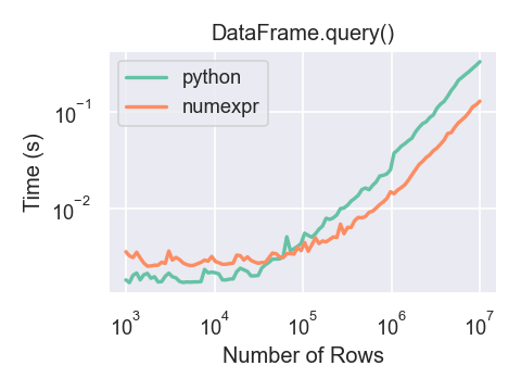
You will only see the performance benefits of using the numexpr engine
with DataFrame.query() if your frame has more than approximately 100,000
rows.
This plot was created using a DataFrame with 3 columns each containing
floating point values generated using numpy.random.randn().
In [302]: df = pd.DataFrame(np.random.randn(8, 4),
   .....:                   index=dates, columns=['A', 'B', 'C', 'D'])
   .....:

In [303]: df2 = df.copy()
Duplicate data#
If you want to identify and remove duplicate rows in a DataFrame, there are
two methods that will help: duplicated and drop_duplicates. Each
takes as an argument the columns to use to identify duplicated rows.
duplicatedreturns a boolean vector whose length is the number of rows, and which indicates whether a row is duplicated.drop_duplicatesremoves duplicate rows.
By default, the first observed row of a duplicate set is considered unique, but
each method has a keep parameter to specify targets to be kept.
keep='first'(default): mark / drop duplicates except for the first occurrence.keep='last': mark / drop duplicates except for the last occurrence.keep=False: mark / drop all duplicates.
In [304]: df2 = pd.DataFrame({'a': ['one', 'one', 'two', 'two', 'two', 'three', 'four'],
   .....:                     'b': ['x', 'y', 'x', 'y', 'x', 'x', 'x'],
   .....:                     'c': np.random.randn(7)})
   .....:

In [305]: df2
Out[305]:
       a  b         c
0    one  x -1.467157
1    one  y  0.113937
2    two  x -1.428572
3    two  y  0.337109
4    two  x  0.052469
5  three  x -2.294560
6   four  x  2.148507

In [306]: df2.duplicated('a')
Out[306]:
0    False
1     True
2    False
3     True
4     True
5    False
6    False
dtype: bool

In [307]: df2.duplicated('a', keep='last')
Out[307]:
0     True
1    False
2     True
3     True
4    False
5    False
6    False
dtype: bool

In [308]: df2.duplicated('a', keep=False)
Out[308]:
0     True
1     True
2     True
3     True
4     True
5    False
6    False
dtype: bool

In [309]: df2.drop_duplicates('a')
Out[309]:
       a  b         c
0    one  x -1.467157
2    two  x -1.428572
5  three  x -2.294560
6   four  x  2.148507

In [310]: df2.drop_duplicates('a', keep='last')
Out[310]:
       a  b         c
1    one  y  0.113937
4    two  x  0.052469
5  three  x -2.294560
6   four  x  2.148507

In [311]: df2.drop_duplicates('a', keep=False)
Out[311]:
       a  b         c
5  three  x -2.294560
6   four  x  2.148507
Also, you can pass a list of columns to identify duplications.
In [312]: df2.duplicated(['a', 'b'])
Out[312]:
0    False
1    False
2    False
3    False
4     True
5    False
6    False
dtype: bool

In [313]: df2.drop_duplicates(['a', 'b'])
Out[313]:
       a  b         c
0    one  x -1.467157
1    one  y  0.113937
2    two  x -1.428572
3    two  y  0.337109
5  three  x -2.294560
6   four  x  2.148507
To drop duplicates by index value, use Index.duplicated then perform slicing.
The same set of options are available for the keep parameter.
In [314]: df3 = pd.DataFrame({'a': np.arange(6),
   .....:                     'b': np.random.randn(6)},
   .....:                    index=['a', 'a', 'b', 'c', 'b', 'a'])
   .....:

In [315]: df3
Out[315]:
   a         b
a  0 -0.293144
a  1 -1.596615
b  2  0.149716
c  3  0.173897
b  4 -0.049440
a  5  1.394590

In [316]: df3.index.duplicated()
Out[316]: array([False,  True, False, False,  True,  True])

In [317]: df3[~df3.index.duplicated()]
Out[317]:
   a         b
a  0 -0.293144
b  2  0.149716
c  3  0.173897

In [318]: df3[~df3.index.duplicated(keep='last')]
Out[318]:
   a         b
c  3  0.173897
b  4 -0.049440
a  5  1.394590

In [319]: df3[~df3.index.duplicated(keep=False)]
Out[319]:
   a         b
c  3  0.173897
Dictionary-like get() method#
Each of Series or DataFrame have a get method which can return a
default value.
In [320]: s = pd.Series([1, 2, 3], index=['a', 'b', 'c'])

In [321]: s.get('a')  # equivalent to s['a']
Out[321]: np.int64(1)

In [322]: s.get('x', default=-1)
Out[322]: -1
Looking up values by index/column labels#
Sometimes you want to extract a set of values given a sequence of row labels
and column labels, this can be achieved by pandas.factorize and NumPy indexing.
For heterogeneous column types, we subset columns to avoid unnecessary NumPy conversions:
def pd_lookup_het(df, row_labels, col_labels):
   rows = df.index.get_indexer(row_labels)
   cols = df.columns.get_indexer(col_labels)
   sub = df.take(np.unique(cols), axis=1)
   sub = sub.take(np.unique(rows), axis=0)
   rows = sub.index.get_indexer(row_labels)
   values = sub.melt()["value"]
   cols = sub.columns.get_indexer(col_labels)
   flat_index = rows + cols * len(sub)
   result = values[flat_index]
   return result
For homogeneous column types, it is fastest to skip column subsetting and go directly to NumPy:
def pd_lookup_hom(df, row_labels, col_labels):
    rows = df.index.get_indexer(row_labels)
    df = df.loc[:, sorted(set(col_labels))]
    cols = df.columns.get_indexer(col_labels)
    result = df.to_numpy()[rows, cols]
    return result
Formerly this could be achieved with the dedicated DataFrame.lookup method
which was deprecated in version 1.2.0 and removed in version 2.0.0.
Index objects#
The pandas Index class and its subclasses can be viewed as
implementing an ordered multiset. Duplicates are allowed.
Index also provides the infrastructure necessary for
lookups, data alignment, and reindexing. The easiest way to create an
Index directly is to pass a list or other sequence to
Index:
In [323]: index = pd.Index(['e', 'd', 'a', 'b'])

In [324]: index
Out[324]: Index(['e', 'd', 'a', 'b'], dtype='str')

In [325]: 'd' in index
Out[325]: True
or using numbers:
In [326]: index = pd.Index([1, 5, 12])

In [327]: index
Out[327]: Index([1, 5, 12], dtype='int64')

In [328]: 5 in index
Out[328]: True
If no dtype is given, Index tries to infer the dtype from the data.
It is also possible to give an explicit dtype when instantiating an Index:
In [329]: index = pd.Index(['e', 'd', 'a', 'b'], dtype="string")

In [330]: index
Out[330]: Index(['e', 'd', 'a', 'b'], dtype='string')

In [331]: index = pd.Index([1, 5, 12], dtype="int8")

In [332]: index
Out[332]: Index([1, 5, 12], dtype='int8')

In [333]: index = pd.Index([1, 5, 12], dtype="float32")

In [334]: index
Out[334]: Index([1.0, 5.0, 12.0], dtype='float32')
You can also pass a name to be stored in the index:
In [335]: index = pd.Index(['e', 'd', 'a', 'b'], name='something')

In [336]: index.name
Out[336]: 'something'
The name, if set, will be shown in the console display:
In [337]: index = pd.Index(list(range(5)), name='rows')

In [338]: columns = pd.Index(['A', 'B', 'C'], name='cols')

In [339]: df = pd.DataFrame(np.random.randn(5, 3), index=index, columns=columns)

In [340]: df
Out[340]:
cols         A         B         C
rows
0     0.698035  0.631397  0.816412
1     0.709404 -1.193616 -0.263520
2    -0.878602  0.035458 -0.285808
3    -0.957431  2.243279 -1.124957
4    -1.994374  0.050270  0.512794

In [341]: df['A']
Out[341]:
rows
0    0.698035
1    0.709404
2   -0.878602
3   -0.957431
4   -1.994374
Name: A, dtype: float64
Setting metadata#
Indexes are “mostly immutable”, but it is possible to set and change their
name attribute. You can use the rename, set_names to set these attributes
directly, and they default to returning a copy.
See Advanced Indexing for usage of MultiIndexes.
In [342]: ind = pd.Index([1, 2, 3])

In [343]: ind.rename("apple")
Out[343]: Index([1, 2, 3], dtype='int64', name='apple')

In [344]: ind
Out[344]: Index([1, 2, 3], dtype='int64')

In [345]: ind = ind.set_names(["apple"])

In [346]: ind.name = "bob"

In [347]: ind
Out[347]: Index([1, 2, 3], dtype='int64', name='bob')
set_names, set_levels, and set_codes also take an optional
level argument
In [348]: index = pd.MultiIndex.from_product([range(3), ['one', 'two']], names=['first', 'second'])

In [349]: index
Out[349]:
MultiIndex([(0, 'one'),
            (0, 'two'),
            (1, 'one'),
            (1, 'two'),
            (2, 'one'),
            (2, 'two')],
           names=['first', 'second'])

In [350]: index.levels[1]
Out[350]: Index(['one', 'two'], dtype='str', name='second')

In [351]: index.set_levels(["a", "b"], level=1)
Out[351]:
MultiIndex([(0, 'a'),
            (0, 'b'),
            (1, 'a'),
            (1, 'b'),
            (2, 'a'),
            (2, 'b')],
           names=['first', 'second'])
Set operations on Index objects#
The two main operations are union and intersection.
Difference is provided via the .difference() method.
In [352]: a = pd.Index(['c', 'b', 'a'])

In [353]: b = pd.Index(['c', 'e', 'd'])

In [354]: a.difference(b)
Out[354]: Index(['a', 'b'], dtype='str')
Also available is the symmetric_difference operation, which returns elements
that appear in either idx1 or idx2, but not in both. This is
equivalent to the Index created by idx1.difference(idx2).union(idx2.difference(idx1)),
with duplicates dropped.
In [355]: idx1 = pd.Index([1, 2, 3, 4])

In [356]: idx2 = pd.Index([2, 3, 4, 5])

In [357]: idx1.symmetric_difference(idx2)
Out[357]: Index([1, 5], dtype='int64')
Note
The resulting index from a set operation will be sorted in ascending order.
When performing Index.union() between indexes with different dtypes, the indexes
must be cast to a common dtype. Typically, though not always, this is object dtype. The
exception is when performing a union between integer and float data. In this case, the
integer values are converted to float
In [358]: idx1 = pd.Index([0, 1, 2])

In [359]: idx2 = pd.Index([0.5, 1.5])

In [360]: idx1.union(idx2)
Out[360]: Index([0.0, 0.5, 1.0, 1.5, 2.0], dtype='float64')
Missing values#
Important
Even though Index can hold missing values (NaN), it should be avoided
if you do not want any unexpected results. For example, some operations
exclude missing values implicitly.
Index.fillna fills missing values with specified scalar value.
In [361]: idx1 = pd.Index([1, np.nan, 3, 4])

In [362]: idx1
Out[362]: Index([1.0, nan, 3.0, 4.0], dtype='float64')

In [363]: idx1.fillna(2)
Out[363]: Index([1.0, 2.0, 3.0, 4.0], dtype='float64')

In [364]: idx2 = pd.DatetimeIndex([pd.Timestamp('2011-01-01'),
   .....:                          pd.NaT,
   .....:                          pd.Timestamp('2011-01-03')])
   .....:

In [365]: idx2
Out[365]:
DatetimeIndex(['2011-01-01', 'NaT', '2011-01-03'], dtype='datetime64[us]',
              freq=None)

In [366]: idx2.fillna(pd.Timestamp('2011-01-02'))
Out[366]:
DatetimeIndex(['2011-01-01', '2011-01-02', '2011-01-03'],
              dtype='datetime64[us]', freq=None)
Set / reset index#
Occasionally you will load or create a data set into a DataFrame and want to add an index after you’ve already done so. There are a couple of different ways.
Set an index#
DataFrame has a set_index() method which takes a column name
(for a regular Index) or a list of column names (for a MultiIndex).
To create a new, re-indexed DataFrame:
In [367]: data = pd.DataFrame({'a': ['bar', 'bar', 'foo', 'foo'],
   .....:                      'b': ['one', 'two', 'one', 'two'],
   .....:                      'c': ['z', 'y', 'x', 'w'],
   .....:                      'd': [1., 2., 3, 4]})
   .....:

In [368]: data
Out[368]:
     a    b  c    d
0  bar  one  z  1.0
1  bar  two  y  2.0
2  foo  one  x  3.0
3  foo  two  w  4.0

In [369]: indexed1 = data.set_index('c')

In [370]: indexed1
Out[370]:
     a    b    d
c
z  bar  one  1.0
y  bar  two  2.0
x  foo  one  3.0
w  foo  two  4.0

In [371]: indexed2 = data.set_index(['a', 'b'])

In [372]: indexed2
Out[372]:
         c    d
a   b
bar one  z  1.0
    two  y  2.0
foo one  x  3.0
    two  w  4.0
The append keyword option allow you to keep the existing index and append
the given columns to a MultiIndex:
In [373]: frame = data.set_index('c', drop=False)

In [374]: frame = frame.set_index(['a', 'b'], append=True)

In [375]: frame
Out[375]:
           c    d
c a   b
z bar one  z  1.0
y bar two  y  2.0
x foo one  x  3.0
w foo two  w  4.0
Other options in set_index allow you not drop the index columns.
In [376]: data.set_index('c', drop=False)
Out[376]:
     a    b  c    d
c
z  bar  one  z  1.0
y  bar  two  y  2.0
x  foo  one  x  3.0
w  foo  two  w  4.0
Reset the index#
As a convenience, there is a new function on DataFrame called
reset_index() which transfers the index values into the
DataFrame’s columns and sets a simple integer index.
This is the inverse operation of set_index().
In [377]: data
Out[377]:
     a    b  c    d
0  bar  one  z  1.0
1  bar  two  y  2.0
2  foo  one  x  3.0
3  foo  two  w  4.0

In [378]: data.reset_index()
Out[378]:
   index    a    b  c    d
0      0  bar  one  z  1.0
1      1  bar  two  y  2.0
2      2  foo  one  x  3.0
3      3  foo  two  w  4.0
The output is more similar to a SQL table or a record array. The names for the
columns derived from the index are the ones stored in the names attribute.
You can use the level keyword to remove only a portion of the index:
In [379]: frame
Out[379]:
           c    d
c a   b
z bar one  z  1.0
y bar two  y  2.0
x foo one  x  3.0
w foo two  w  4.0

In [380]: frame.reset_index(level=1)
Out[380]:
         a  c    d
c b
z one  bar  z  1.0
y two  bar  y  2.0
x one  foo  x  3.0
w two  foo  w  4.0
reset_index takes an optional parameter drop which if true simply
discards the index, instead of putting index values in the DataFrame’s columns.
Adding an ad hoc index#
You can assign a custom index to the index attribute:
In [381]: df_idx = pd.DataFrame(range(4))

In [382]: df_idx.index = pd.Index([10, 20, 30, 40], name="a")

In [383]: df_idx
Out[383]:
    0
a
10  0
20  1
30  2
40  3
Why does assignment fail when using chained indexing?#
Copy-on-Write is the new default with pandas 3.0. This means that chained indexing will never work. See this section for more context.
Series Assignment and Index Alignment#
When assigning a Series to a DataFrame column, pandas performs automatic alignment based on index labels. This is a fundamental behavior that can be surprising to new users who might expect positional assignment.
Key Points:#
Series values are matched to DataFrame rows by index label
Position/order in the Series doesn’t matter
Missing index labels result in NaN values
This behavior is consistent across df[col] = series and df.loc[:, col] = series
You can think of this as reindexing the Series to the DataFrame index before
assignment (for example, df[col] = series.reindex(df.index)).
Examples: .. ipython:: python
import pandas as pd
# Create a DataFrame df = pd.DataFrame({‘values’: [1, 2, 3]}, index=[‘x’, ‘y’, ‘z’])
# Series with matching indices (different order) s1 = pd.Series([10, 20, 30], index=[‘z’, ‘x’, ‘y’]) df[‘aligned’] = s1 # Aligns by index, not position print(df)
# Series with partial index match s2 = pd.Series([100, 200], index=[‘x’, ‘z’]) df[‘partial’] = s2 # Missing ‘y’ gets NaN print(df)
# Series with non-matching indices s3 = pd.Series([1000, 2000], index=[‘a’, ‘b’]) df[‘nomatch’] = s3 # All values become NaN print(df)
#Avoiding Confusion: #If you want positional assignment instead of index alignment: # reset the Series index to match DataFrame index df[‘s1_values’] = s1.reindex(df.index)
Column assignment vs. in-place setting#
While index alignment is consistent between df[col] = value and
df.loc[:, col] = value (see the previous section), the two forms differ in
how they treat the column’s existing dtype:
df[col] = valuereplaces the column. The new column’s dtype is inferred fromvalue, regardless of what dtype the old column had.df.loc[:, col] = value(anddf.iloc[:, i] = value) sets the values in place in the existing column. The original dtype is preserved, and the assignment will raiseTypeErrorifvalueis not compatible with it.
This is most visible for ExtensionDtype columns
such as category, Int64, boolean, or string, where the
replacing form silently drops the extension dtype:
In [384]: df = pd.DataFrame({"a": pd.Categorical(["x", "y"], categories=["x", "y", "z"])})

In [385]: df["a"] = "z"          # replaces the column

In [386]: df.dtypes
Out[386]:
a    str
dtype: object

In [387]: df = pd.DataFrame({"a": pd.Categorical(["x", "y"], categories=["x", "y", "z"])})

In [388]: df.loc[:, "a"] = "z"   # sets values in place

In [389]: df.dtypes
Out[389]:
a    category
dtype: object
The same distinction applies to nullable numeric and boolean dtypes:
In [390]: df = pd.DataFrame({"a": pd.array([1, 2], dtype="Int64")})

In [391]: df["a"] = 5

In [392]: df.dtypes
Out[392]:
a    int64
dtype: object

In [393]: df = pd.DataFrame({"a": pd.array([1, 2], dtype="Int64")})

In [394]: df.loc[:, "a"] = 5

In [395]: df.dtypes
Out[395]:
a    Int64
dtype: object
Use df.loc[:, col] = value (or .iloc) when you want to update every
value of an existing column while keeping its dtype.