Table Visualization

This section demonstrates visualization of tabular data using the Styler class. For information on visualization with charting please see Chart Visualization. This document is written as a Jupyter Notebook, and can be viewed or downloaded here.

Styler Object and Customising the Display

Styling and output display customisation should be performed after the data in a DataFrame has been processed. The Styler is not dynamically updated if further changes to the DataFrame are made. The DataFrame.style attribute is a property that returns a Styler object. It has a _repr_html_ method defined on it so it is rendered automatically in Jupyter Notebook.

The Styler, which can be used for large data but is primarily designed for small data, currently has the ability to output to these formats:

• HTML

• LaTeX

• String (and CSV by extension)

• Excel

• (JSON is not currently available)

The first three of these have display customisation methods designed to format and customise the output. These include:

• Formatting values, the index and columns headers, using .format() and .format_index(),

• Renaming the index or column header labels, using .relabel_index()

• Hiding certain columns, the index and/or column headers, or index names, using .hide()

• Concatenating similar DataFrames, using .concat()

Formatting the Display

Formatting Values

The Styler distinguishes the display value from the actual value, in both data values and index or columns headers. To control the display value, the text is printed in each cell as a string, and we can use the .format() and .format_index() methods to manipulate this according to a format spec string or a callable that takes a single value and returns a string. It is possible to define this for the whole table, or index, or for individual columns, or MultiIndex levels. We can also overwrite index names.

Additionally, the format function has a precision argument to specifically help format floats, as well as decimal and thousands separators to support other locales, an na_rep argument to display missing data, and an escape and hyperlinks arguments to help displaying safe-HTML or safe-LaTeX. The default formatter is configured to adopt pandas’ global options such as styler.format.precision option, controllable using with pd.option_context('format.precision', 2):

import pandas as pd
import numpy as np

df = pd.DataFrame(
    {"strings": ["Adam", "Mike"], "ints": [1, 3], "floats": [1.123, 1000.23]}
)
df.style.format(precision=3, thousands=".", decimal=",").format_index(
    str.upper, axis=1
).relabel_index(["row 1", "row 2"], axis=0)

	STRINGS	INTS	FLOATS
row 1	Adam	1	1,123
row 2	Mike	3	1.000,230

Using Styler to manipulate the display is a useful feature because maintaining the indexing and data values for other purposes gives greater control. You do not have to overwrite your DataFrame to display it how you like. Here is a more comprehensive example of using the formatting functions whilst still relying on the underlying data for indexing and calculations.

weather_df = pd.DataFrame(
    np.random.default_rng().random((10, 2)) * 5,
    index=pd.date_range(start="2021-01-01", periods=10),
    columns=["Tokyo", "Beijing"],
)


def rain_condition(v):
    if v < 1.75:
        return "Dry"
    elif v < 2.75:
        return "Rain"
    return "Heavy Rain"


def make_pretty(styler):
    styler.set_caption("Weather Conditions")
    styler.format(rain_condition)
    styler.format_index(lambda v: v.strftime("%A"))
    styler.background_gradient(axis=None, vmin=1, vmax=5, cmap="YlGnBu")
    return styler


weather_df

	Tokyo	Beijing
2021-01-01	2.351723	4.780392
2021-01-02	4.427868	0.650167
2021-01-03	2.903555	0.016869
2021-01-04	2.026293	2.046236
2021-01-05	2.492046	0.697659
2021-01-06	2.807797	2.848046
2021-01-07	4.105405	1.469667
2021-01-08	0.047884	1.686263
2021-01-09	3.870062	4.501508
2021-01-10	4.578248	4.127059

weather_df.loc["2021-01-04":"2021-01-08"].style.pipe(make_pretty)

Weather Conditions

	Tokyo	Beijing
Monday	Rain	Rain
Tuesday	Rain	Dry
Wednesday	Heavy Rain	Heavy Rain
Thursday	Heavy Rain	Dry
Friday	Dry	Dry

Hiding Data

The index and column headers can be completely hidden, as well subselecting rows or columns that one wishes to exclude. Both these options are performed using the same methods.

The index can be hidden from rendering by calling .hide() without any arguments, which might be useful if your index is integer based. Similarly column headers can be hidden by calling .hide(axis=”columns”) without any further arguments.

Specific rows or columns can be hidden from rendering by calling the same .hide() method and passing in a row/column label, a list-like or a slice of row/column labels to for the subset argument.

Hiding does not change the integer arrangement of CSS classes, e.g. hiding the first two columns of a DataFrame means the column class indexing will still start at col2, since col0 and col1 are simply ignored.

df = pd.DataFrame(np.random.default_rng().standard_normal((5, 5)))
df.style.hide(subset=[0, 2, 4], axis=0).hide(subset=[0, 2, 4], axis=1)

	1	3
1	-0.584283	0.454539
3	0.467254	-0.129875

To invert the function to a show functionality it is best practice to compose a list of hidden items.

show = [0, 2, 4]
df.style.hide([row for row in df.index if row not in show], axis=0).hide(
    [col for col in df.columns if col not in show], axis=1
)

	0	2	4
0	0.535933	0.205277	-0.101159
2	-0.142931	0.683806	1.240106
4	-1.627355	0.510160	1.455765

Concatenating DataFrame Outputs

Two or more Stylers can be concatenated together provided they share the same columns. This is very useful for showing summary statistics for a DataFrame, and is often used in combination with DataFrame.agg.

Since the objects concatenated are Stylers they can independently be styled as will be shown below and their concatenation preserves those styles.

summary_styler = (
    df.agg(["sum", "mean"]).style.format(precision=3).relabel_index(["Sum", "Average"])
)
df.style.format(precision=1).concat(summary_styler)

	0	1	2	3	4
0	0.5	1.5	0.2	0.1	-0.1
1	-2.3	-0.6	1.1	0.5	1.4
2	-0.1	-1.2	0.7	1.3	1.2
3	0.5	0.5	0.5	-0.1	3.0
4	-1.6	-1.7	0.5	0.8	1.5
Sum	-3.078	-1.523	2.928	2.514	6.963
Average	-0.616	-0.305	0.586	0.503	1.393

Styler Object and HTML

The Styler was originally constructed to support the wide array of HTML formatting options. Its HTML output creates an HTML <table> and leverages CSS styling language to manipulate many parameters including colors, fonts, borders, background, etc. See here for more information on styling HTML tables. This allows a lot of flexibility out of the box, and even enables web developers to integrate DataFrames into their existing user interface designs.

Below we demonstrate the default output, which looks very similar to the standard DataFrame HTML representation. But the HTML here has already attached some CSS classes to each cell, even if we haven’t yet created any styles. We can view these by calling the .to_html() method, which returns the raw HTML as string, which is useful for further processing or adding to a file - read on in More about CSS and HTML. This section will also provide a walkthrough for how to convert this default output to represent a DataFrame output that is more communicative. For example how we can build s:

idx = pd.Index(["Tumour (Positive)", "Non-Tumour (Negative)"], name="Actual Label:")
cols = pd.MultiIndex.from_product(
    [["Decision Tree", "Regression", "Random"], ["Tumour", "Non-Tumour"]],
    names=["Model:", "Predicted:"],
)
df = pd.DataFrame(
    [[38.0, 2.0, 18.0, 22.0, 21, np.nan], [19, 439, 6, 452, 226, 232]],
    index=idx,
    columns=cols,
)
df.style

Model:	Decision Tree		Regression		Random
Predicted:	Tumour	Non-Tumour	Tumour	Non-Tumour	Tumour	Non-Tumour
Actual Label:
Tumour (Positive)	38.000000	2.000000	18.000000	22.000000	21	nan
Non-Tumour (Negative)	19.000000	439.000000	6.000000	452.000000	226	232.000000

s

Confusion matrix for multiple cancer prediction models.

Model:	Decision Tree		Regression
Predicted:	Tumour	Non-Tumour	Tumour	Non-Tumour
Actual Label:
Tumour (Positive)	38	2	18	22
Non-Tumour (Negative)	19	439	6	452

The first step we have taken is the create the Styler object from the DataFrame and then select the range of interest by hiding unwanted columns with .hide().

s = df.style.format("{:.0f}").hide(
    [("Random", "Tumour"), ("Random", "Non-Tumour")], axis="columns"
)
s

Model:	Decision Tree		Regression
Predicted:	Tumour	Non-Tumour	Tumour	Non-Tumour
Actual Label:
Tumour (Positive)	38	2	18	22
Non-Tumour (Negative)	19	439	6	452

Methods to Add Styles

There are 3 primary methods of adding custom CSS styles to Styler:

• Using .set_table_styles() to control broader areas of the table with specified internal CSS. Although table styles allow the flexibility to add CSS selectors and properties controlling all individual parts of the table, they are unwieldy for individual cell specifications. Also, note that table styles cannot be exported to Excel.

• Using .set_td_classes() to directly link either external CSS classes to your data cells or link the internal CSS classes created by .set_table_styles(). See here. These cannot be used on column header rows or indexes, and also won’t export to Excel.

• Using the .apply() and .map() functions to add direct internal CSS to specific data cells. See here. As of v1.4.0 there are also methods that work directly on column header rows or indexes: .apply_index() and .map_index(). Note that only these methods add styles that will export to Excel. These methods work in a similar way to DataFrame.apply() and DataFrame.map().

Table Styles

Table styles are flexible enough to control all individual parts of the table, including column headers and indexes. However, they can be unwieldy to type for individual data cells or for any kind of conditional formatting, so we recommend that table styles are used for broad styling, such as entire rows or columns at a time.

Table styles are also used to control features which can apply to the whole table at once such as creating a generic hover functionality. The :hover pseudo-selector, as well as other pseudo-selectors, can only be used this way.

To replicate the normal format of CSS selectors and properties (attribute value pairs), e.g.

tr:hover {
  background-color: #ffff99;
}

the necessary format to pass styles to .set_table_styles() is as a list of dicts, each with a CSS-selector tag and CSS-properties. Properties can either be a list of 2-tuples, or a regular CSS-string, for example:

cell_hover = {  # for row hover use <tr> instead of <td>
    "selector": "td:hover",
    "props": [("background-color", "#ffffb3")],
}
index_names = {
    "selector": ".index_name",
    "props": "font-style: italic; color: darkgrey; font-weight:normal;",
}
headers = {
    "selector": "th:not(.index_name)",
    "props": "background-color: #000066; color: white;",
}
s.set_table_styles([cell_hover, index_names, headers])

Model:	Decision Tree		Regression
Predicted:	Tumour	Non-Tumour	Tumour	Non-Tumour
Actual Label:
Tumour (Positive)	38	2	18	22
Non-Tumour (Negative)	19	439	6	452

Next we just add a couple more styling artifacts targeting specific parts of the table. Be careful here, since we are chaining methods we need to explicitly instruct the method not to overwrite the existing styles.

s.set_table_styles(
    [
        {"selector": "th.col_heading", "props": "text-align: center;"},
        {"selector": "th.col_heading.level0", "props": "font-size: 1.5em;"},
        {"selector": "td", "props": "text-align: center; font-weight: bold;"},
    ],
    overwrite=False,
)

Model:	Decision Tree		Regression
Predicted:	Tumour	Non-Tumour	Tumour	Non-Tumour
Actual Label:
Tumour (Positive)	38	2	18	22
Non-Tumour (Negative)	19	439	6	452

As a convenience method (since version 1.2.0) we can also pass a dict to .set_table_styles() which contains row or column keys. Behind the scenes Styler just indexes the keys and adds relevant .col<m> or .row<n> classes as necessary to the given CSS selectors.

s.set_table_styles(
    {
        ("Regression", "Tumour"): [
            {"selector": "th", "props": "border-left: 1px solid white"},
            {"selector": "td", "props": "border-left: 1px solid #000066"},
        ]
    },
    overwrite=False,
    axis=0,
)

Model:	Decision Tree		Regression
Predicted:	Tumour	Non-Tumour	Tumour	Non-Tumour
Actual Label:
Tumour (Positive)	38	2	18	22
Non-Tumour (Negative)	19	439	6	452

Setting Classes and Linking to External CSS

If you have designed a website then it is likely you will already have an external CSS file that controls the styling of table and cell objects within it. You may want to use these native files rather than duplicate all the CSS in python (and duplicate any maintenance work).

Table Attributes

It is very easy to add a class to the main <table> using .set_table_attributes(). This method can also attach inline styles - read more in CSS Hierarchies.

out = s.set_table_attributes('class="my-table-cls"').to_html()
print(out[out.find("<table") :][:109])

<table id="T_xyz01" class="my-table-cls">
  <thead>
    <tr>
      <th class="index_name level0" >Model:</th>

Data Cell CSS Classes

New in version 1.2.0

The .set_td_classes() method accepts a DataFrame with matching indices and columns to the underlying Styler’s DataFrame. That DataFrame will contain strings as css-classes to add to individual data cells: the <td> elements of the <table>. Rather than use external CSS we will create our classes internally and add them to table style. We will save adding the borders until the section on tooltips.

s.set_table_styles(
    [  # create internal CSS classes
        {"selector": ".true", "props": "background-color: #e6ffe6;"},
        {"selector": ".false", "props": "background-color: #ffe6e6;"},
    ],
    overwrite=False,
)
cell_color = pd.DataFrame(
    [["true ", "false ", "true ", "false "], ["false ", "true ", "false ", "true "]],
    index=df.index,
    columns=df.columns[:4],
)
s.set_td_classes(cell_color)

Model:	Decision Tree		Regression
Predicted:	Tumour	Non-Tumour	Tumour	Non-Tumour
Actual Label:
Tumour (Positive)	38	2	18	22
Non-Tumour (Negative)	19	439	6	452

Styler Functions

Acting on Data

We use the following methods to pass your style functions. Both of those methods take a function (and some other keyword arguments) and apply it to the DataFrame in a certain way, rendering CSS styles.

• .map() (elementwise): accepts a function that takes a single value and returns a string with the CSS attribute-value pair.

• .apply() (column-/row-/table-wise): accepts a function that takes a Series or DataFrame and returns a Series, DataFrame, or numpy array with an identical shape where each element is a string with a CSS attribute-value pair. This method passes each column or row of your DataFrame one-at-a-time or the entire table at once, depending on the axis keyword argument. For columnwise use axis=0, rowwise use axis=1, and for the entire table at once use axis=None.

This method is powerful for applying multiple, complex logic to data cells. We create a new DataFrame to demonstrate this.

df2 = pd.DataFrame(
    np.random.default_rng(0).standard_normal((10, 4)), columns=["A", "B", "C", "D"]
)
df2.style

	A	B	C	D
0	0.125730	-0.132105	0.640423	0.104900
1	-0.535669	0.361595	1.304000	0.947081
2	-0.703735	-1.265421	-0.623274	0.041326
3	-2.325031	-0.218792	-1.245911	-0.732267
4	-0.544259	-0.316300	0.411631	1.042513
5	-0.128535	1.366463	-0.665195	0.351510
6	0.903470	0.094012	-0.743499	-0.921725
7	-0.457726	0.220195	-1.009618	-0.209176
8	-0.159225	0.540846	0.214659	0.355373
9	-0.653829	-0.129614	0.783975	1.493431

For example we can build a function that colors text if it is negative, and chain this with a function that partially fades cells of negligible value. Since this looks at each element in turn we use map.

def style_negative(v, props=""):
    return props if v < 0 else None


s2 = df2.style.map(style_negative, props="color:red;").map(
    lambda v: "opacity: 20%;" if (v < 0.3) and (v > -0.3) else None
)
s2

	A	B	C	D
0	0.125730	-0.132105	0.640423	0.104900
1	-0.535669	0.361595	1.304000	0.947081
2	-0.703735	-1.265421	-0.623274	0.041326
3	-2.325031	-0.218792	-1.245911	-0.732267
4	-0.544259	-0.316300	0.411631	1.042513
5	-0.128535	1.366463	-0.665195	0.351510
6	0.903470	0.094012	-0.743499	-0.921725
7	-0.457726	0.220195	-1.009618	-0.209176
8	-0.159225	0.540846	0.214659	0.355373
9	-0.653829	-0.129614	0.783975	1.493431

We can also build a function that highlights the maximum value across rows, cols, and the DataFrame all at once. In this case we use apply. Below we highlight the maximum in a column.

def highlight_max(s, props=""):
    return np.where(s == np.nanmax(s.values), props, "")


s2.apply(highlight_max, props="color:white;background-color:darkblue", axis=0)

	A	B	C	D
0	0.125730	-0.132105	0.640423	0.104900
1	-0.535669	0.361595	1.304000	0.947081
2	-0.703735	-1.265421	-0.623274	0.041326
3	-2.325031	-0.218792	-1.245911	-0.732267
4	-0.544259	-0.316300	0.411631	1.042513
5	-0.128535	1.366463	-0.665195	0.351510
6	0.903470	0.094012	-0.743499	-0.921725
7	-0.457726	0.220195	-1.009618	-0.209176
8	-0.159225	0.540846	0.214659	0.355373
9	-0.653829	-0.129614	0.783975	1.493431

We can use the same function across the different axes, highlighting here the DataFrame maximum in purple, and row maximums in pink.

s2.apply(highlight_max, props="color:white;background-color:pink;", axis=1).apply(
    highlight_max, props="color:white;background-color:purple", axis=None
)

	A	B	C	D
0	0.125730	-0.132105	0.640423	0.104900
1	-0.535669	0.361595	1.304000	0.947081
2	-0.703735	-1.265421	-0.623274	0.041326
3	-2.325031	-0.218792	-1.245911	-0.732267
4	-0.544259	-0.316300	0.411631	1.042513
5	-0.128535	1.366463	-0.665195	0.351510
6	0.903470	0.094012	-0.743499	-0.921725
7	-0.457726	0.220195	-1.009618	-0.209176
8	-0.159225	0.540846	0.214659	0.355373
9	-0.653829	-0.129614	0.783975	1.493431

This last example shows how some styles have been overwritten by others. In general the most recent style applied is active but you can read more in the section on CSS hierarchies. You can also apply these styles to more granular parts of the DataFrame - read more in section on subset slicing.

It is possible to replicate some of this functionality using just classes but it can be more cumbersome. See item 3) of Optimization

Debugging Tip: If you’re having trouble writing your style function, try just passing it into DataFrame.apply. Internally, Styler.apply uses DataFrame.apply so the result should be the same, and with DataFrame.apply you will be able to inspect the CSS string output of your intended function in each cell.

Acting on the Index and Column Headers

Similar application is achieved for headers by using:

• .map_index() (elementwise): accepts a function that takes a single value and returns a string with the CSS attribute-value pair.

• .apply_index() (level-wise): accepts a function that takes a Series and returns a Series, or numpy array with an identical shape where each element is a string with a CSS attribute-value pair. This method passes each level of your Index one-at-a-time. To style the index use axis=0 and to style the column headers use axis=1.

You can select a level of a MultiIndex but currently no similar subset application is available for these methods.

s2.map_index(lambda v: "color:pink;" if v > 4 else "color:darkblue;", axis=0)
s2.apply_index(
    lambda s: np.where(s.isin(["A", "B"]), "color:pink;", "color:darkblue;"), axis=1
)

	A	B	C	D
0	0.125730	-0.132105	0.640423	0.104900
1	-0.535669	0.361595	1.304000	0.947081
2	-0.703735	-1.265421	-0.623274	0.041326
3	-2.325031	-0.218792	-1.245911	-0.732267
4	-0.544259	-0.316300	0.411631	1.042513
5	-0.128535	1.366463	-0.665195	0.351510
6	0.903470	0.094012	-0.743499	-0.921725
7	-0.457726	0.220195	-1.009618	-0.209176
8	-0.159225	0.540846	0.214659	0.355373
9	-0.653829	-0.129614	0.783975	1.493431

Tooltips and Captions

Table captions can be added with the .set_caption() method. You can use table styles to control the CSS relevant to the caption.

s.set_caption(
    "Confusion matrix for multiple cancer prediction models."
).set_table_styles(
    [{"selector": "caption", "props": "caption-side: bottom; font-size:1.25em;"}],
    overwrite=False,
)

Confusion matrix for multiple cancer prediction models.

Model:	Decision Tree		Regression
Predicted:	Tumour	Non-Tumour	Tumour	Non-Tumour
Actual Label:
Tumour (Positive)	38	2	18	22
Non-Tumour (Negative)	19	439	6	452

Adding tooltips (since version 1.3.0) can be done using the .set_tooltips() method in the same way you can add CSS classes to data cells by providing a string based DataFrame with intersecting indices and columns. You don’t have to specify a css_class name or any css props for the tooltips, since there are standard defaults, but the option is there if you want more visual control.

tt = pd.DataFrame(
    [
        [
            "This model has a very strong true positive rate",
            "This model's total number of false negatives is too high",
        ]
    ],
    index=["Tumour (Positive)"],
    columns=df.columns[[0, 3]],
)
s.set_tooltips(
    tt,
    props="visibility: hidden; position: absolute; z-index: 1; "
    "border: 1px solid #000066;"
    "background-color: white; color: #000066; font-size: 0.8em;"
    "transform: translate(0px, -24px); padding: 0.6em; "
    "border-radius: 0.5em;",
)

Confusion matrix for multiple cancer prediction models.

Model:	Decision Tree		Regression
Predicted:	Tumour	Non-Tumour	Tumour	Non-Tumour
Actual Label:
Tumour (Positive)	38	2	18	22
Non-Tumour (Negative)	19	439	6	452

The only thing left to do for our table is to add the highlighting borders to draw the audience attention to the tooltips. We will create internal CSS classes as before using table styles. Setting classes always overwrites so we need to make sure we add the previous classes.

s.set_table_styles(
    [  # create internal CSS classes
        {"selector": ".border-red", "props": "border: 2px dashed red;"},
        {"selector": ".border-green", "props": "border: 2px dashed green;"},
    ],
    overwrite=False,
)
cell_border = pd.DataFrame(
    [["border-green ", " ", " ", "border-red "], [" ", " ", " ", " "]],
    index=df.index,
    columns=df.columns[:4],
)
s.set_td_classes(cell_color + cell_border)

Confusion matrix for multiple cancer prediction models.

Model:	Decision Tree		Regression
Predicted:	Tumour	Non-Tumour	Tumour	Non-Tumour
Actual Label:
Tumour (Positive)	38	2	18	22
Non-Tumour (Negative)	19	439	6	452

Finer Control with Slicing

The examples we have shown so far for the Styler.apply and Styler.map functions have not demonstrated the use of the subset argument. This is a useful argument which permits a lot of flexibility: it allows you to apply styles to specific rows or columns, without having to code that logic into your style function.

The value passed to subset behaves similar to slicing a DataFrame;

• A scalar is treated as a column label

• A list (or Series or NumPy array) is treated as multiple column labels

• A tuple is treated as (row_indexer, column_indexer)

Consider using pd.IndexSlice to construct the tuple for the last one. We will create a MultiIndexed DataFrame to demonstrate the functionality.

df3 = pd.DataFrame(
    np.random.default_rng().standard_normal((4, 4)),
    pd.MultiIndex.from_product([["A", "B"], ["r1", "r2"]]),
    columns=["c1", "c2", "c3", "c4"],
)
df3

		c1	c2	c3	c4
A	r1	1.322000	-1.853666	-0.159457	1.635827
	r2	1.069083	-0.301842	-0.507852	0.411485
B	r1	-0.120062	0.119718	-0.028951	1.083671
	r2	-1.093112	-0.537696	-1.488655	-0.175511

We will use subset to highlight the maximum in the third and fourth columns with red text. We will highlight the subset sliced region in yellow.

slice_ = ["c3", "c4"]
df3.style.apply(
    highlight_max, props="color:red;", axis=0, subset=slice_
).set_properties(**{"background-color": "#ffffb3"}, subset=slice_)

		c1	c2	c3	c4
A	r1	1.322000	-1.853666	-0.159457	1.635827
	r2	1.069083	-0.301842	-0.507852	0.411485
B	r1	-0.120062	0.119718	-0.028951	1.083671
	r2	-1.093112	-0.537696	-1.488655	-0.175511

If combined with the IndexSlice as suggested then it can index across both dimensions with greater flexibility.

idx = pd.IndexSlice
slice_ = idx[idx[:, "r1"], idx["c2":"c4"]]
df3.style.apply(
    highlight_max, props="color:red;", axis=0, subset=slice_
).set_properties(**{"background-color": "#ffffb3"}, subset=slice_)

		c1	c2	c3	c4
A	r1	1.322000	-1.853666	-0.159457	1.635827
	r2	1.069083	-0.301842	-0.507852	0.411485
B	r1	-0.120062	0.119718	-0.028951	1.083671
	r2	-1.093112	-0.537696	-1.488655	-0.175511

This also provides the flexibility to sub select rows when used with the axis=1.

slice_ = idx[idx[:, "r2"], :]
df3.style.apply(
    highlight_max, props="color:red;", axis=1, subset=slice_
).set_properties(**{"background-color": "#ffffb3"}, subset=slice_)

		c1	c2	c3	c4
A	r1	1.322000	-1.853666	-0.159457	1.635827
	r2	1.069083	-0.301842	-0.507852	0.411485
B	r1	-0.120062	0.119718	-0.028951	1.083671
	r2	-1.093112	-0.537696	-1.488655	-0.175511

There is also scope to provide conditional filtering.

Suppose we want to highlight the maximum across columns 2 and 4 only in the case that the sum of columns 1 and 3 is less than -2.0 (essentially excluding rows (:,'r2')).

slice_ = idx[idx[(df3["c1"] + df3["c3"]) < -2.0], ["c2", "c4"]]
df3.style.apply(
    highlight_max, props="color:red;", axis=1, subset=slice_
).set_properties(**{"background-color": "#ffffb3"}, subset=slice_)

		c1	c2	c3	c4
A	r1	1.322000	-1.853666	-0.159457	1.635827
	r2	1.069083	-0.301842	-0.507852	0.411485
B	r1	-0.120062	0.119718	-0.028951	1.083671
	r2	-1.093112	-0.537696	-1.488655	-0.175511

Only label-based slicing is supported right now, not positional, and not callables.

If your style function uses a subset or axis keyword argument, consider wrapping your function in a functools.partial, partialing out that keyword.

my_func2 = functools.partial(my_func, subset=42)

Optimization

Generally, for smaller tables and most cases, the rendered HTML does not need to be optimized, and we don’t really recommend it. There are two cases where it is worth considering:

• If you are rendering and styling a very large HTML table, certain browsers have performance issues.

• If you are using Styler to dynamically create part of online user interfaces and want to improve network performance.

Here we recommend the following steps to implement:

1. Remove UUID and cell_ids

Ignore the uuid and set cell_ids to False. This will prevent unnecessary HTML.

This is sub-optimal:

df4 = pd.DataFrame([[1, 2], [3, 4]])
s4 = df4.style

This is better:

from pandas.io.formats.style import Styler

s4 = Styler(df4, uuid_len=0, cell_ids=False)

2. Use table styles

Use table styles where possible (e.g. for all cells or rows or columns at a time) since the CSS is nearly always more efficient than other formats.

This is sub-optimal:

props = 'font-family: "Times New Roman", Times, serif; color: #e83e8c; font-size:1.3em;'
df4.style.map(lambda x: props, subset=[1])

	0	1
0	1	2
1	3	4

This is better:

df4.style.set_table_styles([{"selector": "td.col1", "props": props}])

	0	1
0	1	2
1	3	4

3. Set classes instead of using Styler functions

For large DataFrames where the same style is applied to many cells it can be more efficient to declare the styles as classes and then apply those classes to data cells, rather than directly applying styles to cells. It is, however, probably still easier to use the Styler function api when you are not concerned about optimization.

This is sub-optimal:

df2.style.apply(
    highlight_max, props="color:white;background-color:darkblue;", axis=0
).apply(highlight_max, props="color:white;background-color:pink;", axis=1).apply(
    highlight_max, props="color:white;background-color:purple", axis=None
)

	A	B	C	D
0	0.125730	-0.132105	0.640423	0.104900
1	-0.535669	0.361595	1.304000	0.947081
2	-0.703735	-1.265421	-0.623274	0.041326
3	-2.325031	-0.218792	-1.245911	-0.732267
4	-0.544259	-0.316300	0.411631	1.042513
5	-0.128535	1.366463	-0.665195	0.351510
6	0.903470	0.094012	-0.743499	-0.921725
7	-0.457726	0.220195	-1.009618	-0.209176
8	-0.159225	0.540846	0.214659	0.355373
9	-0.653829	-0.129614	0.783975	1.493431

This is better:

build = lambda x: pd.DataFrame(x, index=df2.index, columns=df2.columns)
cls1 = build(df2.apply(highlight_max, props="cls-1 ", axis=0))
cls2 = build(
    df2.apply(highlight_max, props="cls-2 ", axis=1, result_type="expand").values
)
cls3 = build(highlight_max(df2, props="cls-3 "))
df2.style.set_table_styles(
    [
        {"selector": ".cls-1", "props": "color:white;background-color:darkblue;"},
        {"selector": ".cls-2", "props": "color:white;background-color:pink;"},
        {"selector": ".cls-3", "props": "color:white;background-color:purple;"},
    ]
).set_td_classes(cls1 + cls2 + cls3)

	A	B	C	D
0	0.125730	-0.132105	0.640423	0.104900
1	-0.535669	0.361595	1.304000	0.947081
2	-0.703735	-1.265421	-0.623274	0.041326
3	-2.325031	-0.218792	-1.245911	-0.732267
4	-0.544259	-0.316300	0.411631	1.042513
5	-0.128535	1.366463	-0.665195	0.351510
6	0.903470	0.094012	-0.743499	-0.921725
7	-0.457726	0.220195	-1.009618	-0.209176
8	-0.159225	0.540846	0.214659	0.355373
9	-0.653829	-0.129614	0.783975	1.493431

4. Don’t use tooltips

Tooltips require cell_ids to work and they generate extra HTML elements for every data cell.

5. If every byte counts use string replacement

You can remove unnecessary HTML, or shorten the default class names by replacing the default css dict. You can read a little more about CSS below.

my_css = {
    "row_heading": "",
    "col_heading": "",
    "index_name": "",
    "col": "c",
    "row": "r",
    "col_trim": "",
    "row_trim": "",
    "level": "l",
    "data": "",
    "blank": "",
}
html = Styler(df4, uuid_len=0, cell_ids=False)
html.set_table_styles(
    [
        {"selector": "td", "props": props},
        {"selector": ".c1", "props": "color:green;"},
        {"selector": ".l0", "props": "color:blue;"},
    ],
    css_class_names=my_css,
)
print(html.to_html())

<style type="text/css">
#T_ td {
  font-family: "Times New Roman", Times, serif;
  color: #e83e8c;
  font-size: 1.3em;
}
#T_ .c1 {
  color: green;
}
#T_ .l0 {
  color: blue;
}
</style>
<table id="T_">
  <thead>
    <tr>
      <th class=" l0" >&nbsp;</th>
      <th class=" l0 c0" >0</th>
      <th class=" l0 c1" >1</th>
    </tr>
  </thead>
  <tbody>
    <tr>
      <th class=" l0 r0" >0</th>
      <td class=" r0 c0" >1</td>
      <td class=" r0 c1" >2</td>
    </tr>
    <tr>
      <th class=" l0 r1" >1</th>
      <td class=" r1 c0" >3</td>
      <td class=" r1 c1" >4</td>
    </tr>
  </tbody>
</table>

html

	0	1
0	1	2
1	3	4

Builtin Styles

Some styling functions are common enough that we’ve “built them in” to the Styler, so you don’t have to write them and apply them yourself. The current list of such functions is:

• .highlight_null: for use with identifying missing data.

• .highlight_min and .highlight_max: for use with identifying extremities in data.

• .highlight_between and .highlight_quantile: for use with identifying classes within data.

• .background_gradient: a flexible method for highlighting cells based on their, or other, values on a numeric scale.

• .text_gradient: similar method for highlighting text based on their, or other, values on a numeric scale.

• .bar: to display mini-charts within cell backgrounds.

The individual documentation on each function often gives more examples of their arguments.

Highlight Null

df2.iloc[0, 2] = np.nan
df2.iloc[4, 3] = np.nan
df2.loc[:4].style.highlight_null(color="yellow")

	A	B	C	D
0	0.125730	-0.132105	nan	0.104900
1	-0.535669	0.361595	1.304000	0.947081
2	-0.703735	-1.265421	-0.623274	0.041326
3	-2.325031	-0.218792	-1.245911	-0.732267
4	-0.544259	-0.316300	0.411631	nan

Highlight Min or Max

df2.loc[:4].style.highlight_max(
    axis=1, props=("color:white; " "font-weight:bold; " "background-color:darkblue;")
)

	A	B	C	D
0	0.125730	-0.132105	nan	0.104900
1	-0.535669	0.361595	1.304000	0.947081
2	-0.703735	-1.265421	-0.623274	0.041326
3	-2.325031	-0.218792	-1.245911	-0.732267
4	-0.544259	-0.316300	0.411631	nan

Highlight Between

This method accepts ranges as float, or NumPy arrays or Series provided the indexes match.

left = pd.Series([1.0, 0.0, 1.0], index=["A", "B", "D"])
df2.loc[:4].style.highlight_between(
    left=left, right=1.5, axis=1, props="color:white; background-color:purple;"
)

	A	B	C	D
0	0.125730	-0.132105	nan	0.104900
1	-0.535669	0.361595	1.304000	0.947081
2	-0.703735	-1.265421	-0.623274	0.041326
3	-2.325031	-0.218792	-1.245911	-0.732267
4	-0.544259	-0.316300	0.411631	nan

Highlight Quantile

Useful for detecting the highest or lowest percentile values

df2.loc[:4].style.highlight_quantile(q_left=0.85, axis=None, color="yellow")

	A	B	C	D
0	0.125730	-0.132105	nan	0.104900
1	-0.535669	0.361595	1.304000	0.947081
2	-0.703735	-1.265421	-0.623274	0.041326
3	-2.325031	-0.218792	-1.245911	-0.732267
4	-0.544259	-0.316300	0.411631	nan

Background Gradient and Text Gradient

You can create “heatmaps” with the background_gradient and text_gradient methods. These require matplotlib, and we’ll use Seaborn to get a nice colormap.

import seaborn as sns

cm = sns.light_palette("green", as_cmap=True)

df2.style.background_gradient(cmap=cm)

	A	B	C	D
0	0.125730	-0.132105	nan	0.104900
1	-0.535669	0.361595	1.304000	0.947081
2	-0.703735	-1.265421	-0.623274	0.041326
3	-2.325031	-0.218792	-1.245911	-0.732267
4	-0.544259	-0.316300	0.411631	nan
5	-0.128535	1.366463	-0.665195	0.351510
6	0.903470	0.094012	-0.743499	-0.921725
7	-0.457726	0.220195	-1.009618	-0.209176
8	-0.159225	0.540846	0.214659	0.355373
9	-0.653829	-0.129614	0.783975	1.493431

df2.style.text_gradient(cmap=cm)

	A	B	C	D
0	0.125730	-0.132105	nan	0.104900
1	-0.535669	0.361595	1.304000	0.947081
2	-0.703735	-1.265421	-0.623274	0.041326
3	-2.325031	-0.218792	-1.245911	-0.732267
4	-0.544259	-0.316300	0.411631	nan
5	-0.128535	1.366463	-0.665195	0.351510
6	0.903470	0.094012	-0.743499	-0.921725
7	-0.457726	0.220195	-1.009618	-0.209176
8	-0.159225	0.540846	0.214659	0.355373
9	-0.653829	-0.129614	0.783975	1.493431

.background_gradient and .text_gradient have a number of keyword arguments to customise the gradients and colors. See the documentation.

Set properties

Use Styler.set_properties when the style doesn’t actually depend on the values. This is just a simple wrapper for .map where the function returns the same properties for all cells.

df2.loc[:4].style.set_properties(
    **{"background-color": "black", "color": "lawngreen", "border-color": "white"}
)

	A	B	C	D
0	0.125730	-0.132105	nan	0.104900
1	-0.535669	0.361595	1.304000	0.947081
2	-0.703735	-1.265421	-0.623274	0.041326
3	-2.325031	-0.218792	-1.245911	-0.732267
4	-0.544259	-0.316300	0.411631	nan

Bar charts

You can include “bar charts” in your DataFrame.

df2.style.bar(subset=["A", "B"], color="#d65f5f")

	A	B	C	D
0	0.125730	-0.132105	nan	0.104900
1	-0.535669	0.361595	1.304000	0.947081
2	-0.703735	-1.265421	-0.623274	0.041326
3	-2.325031	-0.218792	-1.245911	-0.732267
4	-0.544259	-0.316300	0.411631	nan
5	-0.128535	1.366463	-0.665195	0.351510
6	0.903470	0.094012	-0.743499	-0.921725
7	-0.457726	0.220195	-1.009618	-0.209176
8	-0.159225	0.540846	0.214659	0.355373
9	-0.653829	-0.129614	0.783975	1.493431

Additional keyword arguments give more control on centering and positioning, and you can pass a list of [color_negative, color_positive] to highlight lower and higher values or a matplotlib colormap.

To showcase an example here’s how you can change the above with the new align option, combined with setting vmin and vmax limits, the width of the figure, and underlying css props of cells, leaving space to display the text and the bars. We also use text_gradient to color the text the same as the bars using a matplotlib colormap (although in this case the visualization is probably better without this additional effect).

df2.style.format("{:.3f}", na_rep="").bar(
    align=0,
    vmin=-2.5,
    vmax=2.5,
    cmap="bwr",
    height=50,
    width=60,
    props="width: 120px; border-right: 1px solid black;",
).text_gradient(cmap="bwr", vmin=-2.5, vmax=2.5)

	A	B	C	D
0	0.126	-0.132		0.105
1	-0.536	0.362	1.304	0.947
2	-0.704	-1.265	-0.623	0.041
3	-2.325	-0.219	-1.246	-0.732
4	-0.544	-0.316	0.412
5	-0.129	1.366	-0.665	0.352
6	0.903	0.094	-0.743	-0.922
7	-0.458	0.220	-1.010	-0.209
8	-0.159	0.541	0.215	0.355
9	-0.654	-0.130	0.784	1.493

The following example aims to give a highlight of the behavior of the new align options:

HTML(head)

Align	All Negative	Both Neg and Pos	All Positive	Large Positive
left	-100 -60 -30 -20	-10 -5 0 90	10 20 50 100	100 103 101 102
right	-100 -60 -30 -20	-10 -5 0 90	10 20 50 100	100 103 101 102
zero	-100 -60 -30 -20	-10 -5 0 90	10 20 50 100	100 103 101 102
mid	-100 -60 -30 -20	-10 -5 0 90	10 20 50 100	100 103 101 102
mean	-100 -60 -30 -20	-10 -5 0 90	10 20 50 100	100 103 101 102
99	-100 -60 -30 -20	-10 -5 0 90	10 20 50 100	100 103 101 102

Sharing styles

Say you have a lovely style built up for a DataFrame, and now you want to apply the same style to a second DataFrame. Export the style with df1.style.export, and import it on the second DataFrame with df1.style.set

style1 = (
    df2.style.map(style_negative, props="color:red;")
    .map(lambda v: "opacity: 20%;" if (v < 0.3) and (v > -0.3) else None)
    .set_table_styles([{"selector": "th", "props": "color: blue;"}])
    .hide(axis="index")
)
style1

A	B	C	D
0.125730	-0.132105	nan	0.104900
-0.535669	0.361595	1.304000	0.947081
-0.703735	-1.265421	-0.623274	0.041326
-2.325031	-0.218792	-1.245911	-0.732267
-0.544259	-0.316300	0.411631	nan
-0.128535	1.366463	-0.665195	0.351510
0.903470	0.094012	-0.743499	-0.921725
-0.457726	0.220195	-1.009618	-0.209176
-0.159225	0.540846	0.214659	0.355373
-0.653829	-0.129614	0.783975	1.493431

style2 = df3.style
style2.use(style1.export())
style2

c1	c2	c3	c4
1.322000	-1.853666	-0.159457	1.635827
1.069083	-0.301842	-0.507852	0.411485
-0.120062	0.119718	-0.028951	1.083671
-1.093112	-0.537696	-1.488655	-0.175511

Notice that you’re able to share the styles even though they’re data aware. The styles are re-evaluated on the new DataFrame they’ve been used upon.

Limitations

• DataFrame only (use Series.to_frame().style)

• The index and columns do not need to be unique, but certain styling functions can only work with unique indexes.

• No large repr, and construction performance isn’t great; although we have some HTML optimizations

• You can only apply styles, you can’t insert new HTML entities, except via subclassing.

Other Fun and Useful Stuff

Here are a few interesting examples.

Widgets

Styler interacts pretty well with widgets. If you’re viewing this online instead of running the notebook yourself, you’re missing out on interactively adjusting the color palette.

from ipywidgets import widgets


@widgets.interact
def f(h_neg=(0, 359, 1), h_pos=(0, 359), s=(0.0, 99.9), l_post=(0.0, 99.9)):
    return df2.style.background_gradient(
        cmap=sns.palettes.diverging_palette(
            h_neg=h_neg, h_pos=h_pos, s=s, l=l_post, as_cmap=True
        )
    )

Magnify

def magnify():
    return [
        {"selector": "th", "props": [("font-size", "4pt")]},
        {"selector": "td", "props": [("padding", "0em 0em")]},
        {"selector": "th:hover", "props": [("font-size", "12pt")]},
        {
            "selector": "tr:hover td:hover",
            "props": [("max-width", "200px"), ("font-size", "12pt")],
        },
    ]

cmap = sns.diverging_palette(5, 250, as_cmap=True)
bigdf = pd.DataFrame(np.random.default_rng(25).standard_normal((20, 25))).cumsum()

bigdf.style.background_gradient(cmap, axis=1).set_properties(
    **{"max-width": "80px", "font-size": "1pt"}
).set_caption("Hover to magnify").format(precision=2).set_table_styles(magnify())

Hover to magnify

	0	1	2	3	4	5	6	7	8	9	10	11	12	13	14	15	16	17	18	19	20	21	22	23	24
0	0.35	-0.00	-0.53	-2.28	0.02	0.93	1.04	-0.54	2.23	1.94	-0.23	-0.16	0.96	-0.25	0.22	1.22	1.19	-0.53	-0.46	-0.55	-0.01	0.07	-0.39	0.77	0.05
1	0.37	-1.97	-1.92	-2.97	0.38	0.06	2.60	-0.39	2.49	2.06	0.26	0.77	0.41	1.31	-0.55	1.74	0.98	-0.70	0.21	-0.35	1.59	-0.43	0.13	1.36	2.16
2	1.98	-1.27	-0.24	-2.12	-0.40	0.39	3.83	-0.91	4.01	2.42	-0.36	1.23	-1.16	0.62	-1.60	2.24	-0.04	-2.26	0.52	-0.83	0.87	-1.03	1.17	1.53	1.41
3	4.78	-0.78	1.67	-1.07	0.96	-0.48	3.26	-0.27	3.93	2.50	0.72	-1.07	-1.49	2.16	-2.07	2.28	0.34	-1.94	0.83	-1.76	1.20	-1.63	2.75	0.90	1.67
4	4.58	0.35	1.79	-0.36	0.40	-0.86	2.31	-0.44	3.65	1.36	-0.53	-0.91	-1.67	1.45	-2.99	1.17	0.44	-2.48	0.20	-2.32	0.73	-1.94	2.84	-0.86	1.41
5	3.38	-0.02	3.04	-2.28	-0.89	-1.38	0.01	1.95	3.01	2.98	-0.62	0.27	-0.86	1.15	-2.49	0.51	-0.04	-0.99	-0.67	-3.24	3.28	-2.33	3.14	0.78	0.92
6	2.81	1.80	3.02	-2.01	-1.23	-0.85	-1.57	2.12	4.01	3.94	-1.13	0.91	1.28	1.27	-1.81	0.15	-1.77	-0.25	-1.63	-3.94	3.34	-2.35	3.01	1.90	1.05
7	2.85	0.72	3.92	-3.29	-3.49	-1.67	-0.87	2.46	5.28	4.34	-0.76	1.24	0.64	0.81	-2.27	0.34	-2.71	-0.67	-1.35	-4.01	3.06	-2.55	1.78	0.54	0.25
8	3.80	1.51	4.19	-2.67	-2.71	-4.04	-1.42	3.30	7.04	4.52	0.96	2.40	0.78	-0.24	-3.28	0.28	-2.51	-0.74	-0.74	-3.44	3.11	-2.12	2.07	-1.35	-1.03
9	4.11	2.27	4.29	-2.97	-2.50	-3.58	-1.25	1.32	7.36	5.25	1.08	4.60	-0.64	-2.05	0.09	-0.72	-4.96	-1.31	0.09	-4.16	2.68	-1.37	4.02	-0.59	-0.72
10	3.67	3.02	7.08	-4.10	-3.57	-3.95	-0.53	1.94	7.14	4.78	2.44	5.06	0.69	-2.28	1.23	-1.56	-2.90	-1.71	-0.27	-3.72	2.50	-1.97	4.47	-1.23	1.21
11	2.98	3.85	6.33	-5.84	-5.90	-3.91	-1.94	2.08	6.33	4.70	2.41	6.84	0.50	-3.68	-1.10	-0.67	-2.80	-0.28	-1.88	-3.91	1.67	-1.48	4.15	0.17	0.79
12	2.76	3.21	6.80	-4.75	-5.36	-4.53	-3.00	1.17	6.52	4.20	2.25	7.97	0.98	-3.45	-1.59	-0.86	-3.09	-0.24	-2.08	-3.73	1.03	-0.18	4.54	0.48	1.69
13	1.69	2.02	5.31	-5.51	-4.79	-4.34	-1.42	-0.24	6.96	2.92	0.97	6.70	2.18	-3.38	-0.33	-0.77	-2.39	0.42	-1.53	-3.59	1.98	0.01	4.61	0.52	1.11
14	0.17	1.26	7.10	-5.35	-5.81	-4.61	-0.45	1.61	5.10	1.31	-1.18	6.09	1.25	-2.23	0.32	-1.33	-0.08	-0.19	-1.21	-2.83	0.97	0.13	4.89	0.36	1.83
15	0.01	0.61	7.94	-5.85	-5.35	-5.10	0.14	1.76	3.89	1.72	-1.61	7.86	0.71	-1.38	-1.95	-1.84	-1.88	-0.14	-2.02	-1.45	1.68	1.62	3.97	-1.88	1.80
16	1.42	0.91	9.86	-6.10	-6.02	-4.56	1.24	1.38	3.25	1.05	0.38	5.77	1.92	-1.51	-0.36	-1.01	-3.01	0.10	-2.50	-1.99	0.29	2.91	2.07	-1.64	3.87
17	1.94	2.55	10.78	-4.77	-6.87	-4.38	1.74	1.63	2.34	0.06	0.41	6.21	2.20	-3.13	-0.88	-1.57	-2.59	-0.76	-2.38	-3.21	-0.11	3.62	2.91	-2.87	3.98
18	1.27	4.45	11.25	-4.68	-4.93	-7.30	0.92	2.30	2.34	0.52	-0.15	6.01	2.52	-1.89	1.37	-2.65	-1.98	-2.85	-2.78	-2.81	-0.86	3.93	2.83	-1.04	4.17
19	0.72	2.89	10.94	-3.85	-2.50	-7.04	0.77	2.27	2.83	1.63	0.94	6.26	3.07	-1.99	2.65	-4.04	-0.91	-2.69	-2.70	-2.49	-0.86	3.16	2.88	-0.85	4.54

Sticky Headers

If you display a large matrix or DataFrame in a notebook, but you want to always see the column and row headers you can use the .set_sticky method which manipulates the table styles CSS.

bigdf = pd.DataFrame(np.random.default_rng().standard_normal((16, 100)))
bigdf.style.set_sticky(axis="index")

	0	1	2	3	4	5	6	7	8	9	10	11	12	13	14	15	16	17	18	19	20	21	22	23	24	25	26	27	28	29	30	31	32	33	34	35	36	37	38	39	40	41	42	43	44	45	46	47	48	49	50	51	52	53	54	55	56	57	58	59	60	61	62	63	64	65	66	67	68	69	70	71	72	73	74	75	76	77	78	79	80	81	82	83	84	85	86	87	88	89	90	91	92	93	94	95	96	97	98	99
0	-0.171120	0.082320	-0.015076	-0.862761	-0.424560	-0.335949	0.085080	0.079596	-1.087363	0.994491	0.538135	2.402538	-2.307707	-0.266009	-0.282398	0.237444	-0.419995	1.362133	1.370810	-0.103477	-0.170310	-0.817436	-0.066509	2.026355	-0.510020	-1.830264	-0.131227	1.053328	0.739997	-1.399279	0.436862	1.872572	0.540978	0.098412	0.270673	-0.693201	-1.671970	1.367258	-1.116426	0.071711	-0.501040	-0.381561	0.542268	-0.221593	0.731642	-1.089058	-0.649875	1.830443	-0.385249	-0.147615	-0.129617	0.860898	1.597305	-0.977332	2.271532	1.202568	0.416666	-0.594970	-0.854145	1.907710	0.165570	0.107243	-0.834453	-0.088095	0.277615	-0.330419	-0.464735	-0.011937	-0.174652	0.293430	-0.493227	-0.380206	-1.439229	1.209757	1.701451	-1.887625	1.469170	0.355522	-1.104089	-2.667238	-0.137117	0.837252	-0.607505	0.951665	-1.428459	-0.088456	-0.376275	0.809469	0.702644	-0.740375	-0.802472	-0.052354	0.544894	0.968257	-0.604576	0.613034	1.272415	-0.256237	-0.920144	0.265003
1	-0.663018	-0.333494	-0.425423	-1.022124	0.687989	-1.355117	1.034644	0.049582	-0.721685	-0.299087	0.577043	0.360842	0.136424	0.678275	-1.542764	1.041152	-0.449859	0.465490	-0.863124	-2.408665	0.265037	1.922575	-0.023019	-0.411215	-1.310369	-2.101395	0.593825	-0.704423	-0.096204	2.323237	-0.115810	-0.894426	0.096662	-2.419395	-0.250394	0.095282	0.067893	-0.565723	-1.645417	-1.376456	-0.982831	-0.159220	-0.177820	-0.190759	-2.585100	0.353131	-0.076633	-0.983959	0.747156	-0.693932	1.599877	-1.929582	0.450544	-0.581506	-1.672558	2.137992	0.132794	-1.138771	0.415835	0.481424	-1.157342	1.100410	1.950182	-1.128543	-0.325662	-0.280321	0.212310	-0.188585	-0.976608	-1.516561	0.163003	-2.333685	2.100946	-0.800227	1.478007	-0.699633	0.163939	-0.425398	1.373529	0.088711	0.736041	-1.809644	0.737645	1.592360	0.378306	-1.809835	0.397836	-0.100436	-1.453637	-0.234894	-1.131668	1.097259	0.585642	0.079932	-0.478904	-1.030162	-0.003831	1.297403	-2.505450	0.541754
2	0.079948	0.402550	0.050950	0.959884	-1.181454	0.853630	0.323620	-0.375012	-0.069608	-0.005153	-1.740715	0.270255	1.406421	-0.259662	-0.256742	-0.340615	1.058275	1.294904	0.514233	1.448319	0.211709	0.729058	0.253114	0.969415	-0.423722	-1.572842	1.065800	-0.050361	0.016031	0.899770	-2.825028	-0.333058	-0.590798	0.969483	0.906278	1.290511	-1.210255	-1.466437	-0.254611	0.727389	0.078240	0.226361	0.559705	0.669053	-0.322721	-2.198479	0.690678	-0.356816	-0.867903	-0.937059	0.406752	-1.708655	0.052858	0.665169	-0.433447	0.674931	0.673780	-0.818268	-0.842258	-1.383710	-0.826188	0.582393	-1.114504	0.662123	-1.562780	-1.499154	-0.987593	0.777186	-1.127848	-1.859546	0.041910	-0.403520	-1.171240	1.482575	-0.200220	1.137589	0.661952	-1.666052	-1.306012	-0.485832	-0.958661	-0.839218	0.829636	1.125905	-0.867266	0.460070	0.409786	0.624908	0.900411	-0.728128	0.746620	-1.523548	-1.658839	0.220686	0.352058	1.620696	0.573615	0.329953	0.579977	-0.238289
3	-0.360552	-1.331369	-0.808421	-0.112649	0.238842	-0.017897	-0.939260	-1.696166	-0.338132	-0.770661	-1.336905	0.059935	0.256959	0.020487	-0.065045	-0.231370	0.533890	-1.501946	0.103279	0.508774	0.684896	0.152134	-0.132853	0.124360	-1.399220	0.963862	-0.157068	-1.229154	-0.651267	-1.376211	-0.190904	-1.977200	-0.526107	1.065597	-0.210207	0.714524	0.298872	-1.076300	0.520563	-0.678111	-0.499750	-1.135148	-1.335407	0.458488	-0.573996	-0.181243	-0.447595	-0.491511	0.097197	0.039836	0.167484	-2.211661	0.608466	1.076215	-0.432191	2.199082	-1.100062	0.993823	0.136829	-0.218229	0.056178	-0.543637	-1.613595	0.066149	0.062044	1.029812	-1.696570	-0.115148	-0.070998	1.553803	-0.493876	-1.287044	-0.012841	0.294867	1.073476	0.077991	0.872603	-0.978575	0.166653	0.144585	-1.081555	-0.706486	-0.331649	-0.647228	-0.158331	0.542114	0.342348	-0.064516	0.169187	0.702900	1.329567	-0.843355	0.661349	-0.971124	-0.047263	-0.282450	1.358599	-0.887310	0.237673	-0.931564
4	-2.386699	-0.937011	0.007113	1.758812	-0.832762	-0.587146	0.401495	-0.178789	0.741643	0.347012	1.317754	0.552158	-0.616103	-0.073845	-1.415015	-0.169030	-1.164888	0.637948	-0.957969	0.166858	0.467709	0.716331	1.097221	0.544002	-2.491872	-0.217335	0.555904	1.809462	0.546924	0.397597	-1.437441	1.618733	-0.631699	-1.045940	-0.254221	-0.468257	0.738282	-0.731354	-0.456130	0.527798	-1.376907	0.500520	0.631979	-2.016671	0.071787	-0.752886	-0.170110	0.565714	-0.171605	0.405947	-0.617434	-2.600459	-0.202214	-0.978805	0.079428	2.469205	-0.631417	-0.192087	0.601784	-0.806189	1.055625	-0.419505	-0.929344	-1.324801	0.679576	0.023773	-1.517802	-0.974390	0.861118	-0.100048	-0.580625	-0.963020	2.857922	0.857042	0.505642	-0.536282	-0.238396	-0.898890	1.151407	0.404703	-0.013223	1.009208	0.271684	-1.168553	-0.434361	-0.655993	2.158729	-0.845701	2.259306	0.936815	1.109472	-1.098217	0.489439	-0.695511	-0.823820	0.538490	-0.012931	-0.331585	-0.629779	-0.246929
5	-1.099854	0.784069	-0.168901	0.190662	-0.874833	2.215354	-0.617582	-0.177713	-1.759845	-2.026917	-0.065430	-0.220466	-0.573668	-0.551487	-0.373323	-0.276321	-0.143232	-0.480025	1.728644	-1.309899	-0.067923	-1.759922	0.715373	1.387737	-0.573310	0.754037	2.687766	-0.029470	0.843975	-0.228963	0.055624	-0.276441	0.623661	-1.782516	-0.565546	0.483264	-0.128074	-0.386776	0.466557	1.770411	2.187306	0.393372	-1.352593	-0.275751	1.896815	0.067230	-0.056926	-2.195040	0.896650	-0.081725	1.004220	0.258347	1.362914	0.079839	0.337755	0.614527	-0.350323	0.675699	1.024361	1.264855	-0.115577	1.689455	1.853121	0.717956	-0.292563	0.290890	1.830459	0.000020	1.290355	2.539225	-0.170931	1.071190	0.428511	-1.868380	0.006405	0.591451	-2.307273	0.197780	-0.048375	-0.233134	0.193173	0.098082	-0.580129	-1.436661	-0.105554	-0.092528	0.548947	1.599073	0.273379	-0.344253	0.533470	0.389709	-0.884572	2.318954	-0.193356	0.328749	0.208747	-0.679755	-1.319677	0.819993
6	1.763441	0.206581	-0.000883	-1.238988	-0.953071	-1.274202	-0.263042	0.877862	0.488130	-0.408415	-0.276975	0.044332	0.108241	0.391976	2.050306	-0.144287	0.293056	0.739188	-1.400728	0.055724	0.181260	-0.318387	0.748465	-0.194547	0.146858	-1.633308	0.124250	-0.531895	0.025639	0.493592	-0.712113	0.103961	1.464789	0.211251	-1.821982	1.861475	1.181012	0.985207	-0.665876	-0.666292	2.017589	-0.247838	-0.208413	0.167947	-0.246040	1.574797	-1.361839	-0.679408	-0.232750	0.078497	-0.822830	-1.932769	-1.321052	-0.674640	-0.413226	-0.849700	-0.065091	-0.572528	-0.589007	-0.979777	1.100834	-0.225404	0.517349	-0.192950	-0.807750	-0.515138	1.218431	0.531596	1.004456	-0.571406	0.601067	0.505421	-0.796555	1.253455	-0.105680	1.445231	1.000925	-0.326597	-1.206628	-1.152409	-0.476332	-0.514340	-0.323526	0.338528	-0.778724	-0.369783	-1.118515	0.832346	-0.038038	0.312934	-1.273896	0.966414	1.330135	-0.357181	0.232750	-0.149090	0.189198	0.406334	-0.942040	0.459327
7	0.184823	1.186374	0.423597	-0.843396	0.288892	-0.514854	-0.429357	-0.312087	-0.086789	-0.550485	-0.021475	-0.824428	0.698034	2.629851	1.629515	0.303322	0.261515	-0.775321	-0.060611	-2.886863	1.241624	0.138706	0.690738	-0.356225	-0.509767	-0.361752	0.709567	-0.531357	-0.429430	0.627381	0.281410	0.168911	0.898122	-0.158154	0.951927	0.138292	-1.937625	-0.786370	-0.369731	0.273769	-0.572598	-0.289341	-0.381009	-0.570746	-0.401716	-1.396368	0.769835	0.528153	-0.030596	-0.165872	-0.283821	-0.322214	-0.624404	-2.242681	1.674467	-0.264027	0.907928	-0.575276	0.605758	-0.785597	1.231176	1.162602	0.073809	-1.548027	-0.295748	0.930394	-0.804564	-1.054638	1.482988	0.408792	-0.470632	1.393740	-0.292784	-0.364993	-0.600312	0.293323	1.562652	1.496533	-0.035166	-0.519372	-0.108322	0.523266	1.538140	1.041437	0.980739	-0.052248	1.439454	0.653643	-0.979750	0.720695	1.040935	-0.861497	0.506927	1.107212	0.275161	-0.977082	0.347323	0.731328	0.663211	0.547771
8	-1.544061	0.802588	-1.281983	-0.100855	-0.446214	0.597910	1.752483	-0.600458	-0.128884	0.834686	-0.262974	0.704269	-1.509827	-1.496822	0.347779	0.718217	-1.410954	-1.955808	0.629878	-0.349222	1.922397	-0.623952	-1.149572	-1.435311	0.016041	0.746193	-0.308201	-0.851956	-2.852554	-1.888903	-0.553378	0.413015	0.933527	-0.467705	0.453923	-0.590037	1.272636	-0.817616	0.468221	1.638105	2.483751	0.380952	-1.482743	0.871765	-0.298175	0.492777	0.662677	-0.594538	0.733115	-1.640682	0.482834	0.207139	2.161863	0.210512	1.015685	-1.256434	0.330753	0.811411	0.599824	-1.291534	-1.399262	0.394095	0.266774	1.521544	0.812533	0.064935	-0.449277	0.519873	1.052251	-0.184506	1.384171	1.170852	-0.005942	-0.782596	-2.652286	-0.283522	0.607344	-0.178338	0.459114	0.655403	0.048122	1.273647	-0.182727	2.905705	-0.913660	0.356620	-0.033687	1.546893	-1.539991	0.131022	-0.465941	0.222973	0.077891	-0.440143	0.638600	-0.577189	-1.122749	0.615366	-1.019398	-0.947037
9	0.994208	-0.253817	-0.403260	1.517921	0.409642	0.279115	1.100896	-0.182414	0.288794	0.786611	-0.048654	-0.063618	0.596182	0.569012	-0.159818	-2.320942	0.548098	-1.027066	-0.259585	0.827921	-0.963361	-0.224631	1.063497	-1.295343	-1.336773	-0.090650	0.386013	0.246620	0.053025	-1.161174	1.218824	-0.603278	-0.851747	0.714409	0.179378	0.933773	-1.603374	-0.558057	-0.206977	2.571327	-0.314964	-1.990119	1.365246	-0.329209	1.209783	-0.613605	1.881957	2.016206	-0.265782	-0.141482	-3.134931	1.537799	0.788622	0.564998	1.760180	-0.870712	-0.533960	1.305646	-1.899284	1.131938	0.919342	1.977196	-1.183698	0.538904	0.845296	1.189494	1.110759	-2.704513	-0.373397	0.579398	-0.860382	-0.604267	-0.190463	-0.241159	0.022940	0.905027	-0.578822	-1.173097	0.517861	1.237915	-0.602740	0.670181	0.001183	0.442170	-0.194734	-0.683431	0.796713	2.044331	0.448948	-2.241439	1.193300	-0.041337	0.131785	-0.752452	-0.390518	-1.778382	-0.502282	-1.242683	-1.536029	1.003322
10	-0.748647	-1.142438	-0.539436	1.585855	-0.566590	0.388746	1.962302	-0.519004	-0.116942	0.378698	-0.454755	-0.828458	0.500907	-0.272635	2.449549	-0.506236	0.981879	-0.812782	-0.822548	-0.010896	2.183000	-0.676791	-1.319908	0.110130	0.380739	0.393422	-0.752694	0.866836	0.372462	-1.087262	0.298225	0.544792	0.435774	-0.031238	0.589594	1.857035	1.677708	0.001208	0.044026	0.577536	-0.241303	-0.480287	-0.550225	1.341058	-1.193717	-0.645023	1.232698	-0.811766	0.220187	0.735327	-0.671222	0.369166	-0.330114	-1.354303	-2.058791	0.358430	2.210960	0.582215	-0.103244	2.016446	-0.665865	-0.391315	0.444274	1.223269	-1.302005	0.116181	-1.410425	0.453411	0.198611	1.719831	0.277251	-0.461945	-0.162147	0.145688	0.289667	-2.337579	1.648394	0.617246	-0.265736	0.614119	0.391728	-1.337620	1.726695	-0.871533	1.285731	0.614193	0.224791	-0.620758	1.365524	2.220693	0.140085	-1.464040	0.367303	0.167120	0.130021	0.927258	-0.668873	0.369374	-0.517055	-1.036274
11	0.375593	-1.020335	0.757797	0.038024	0.869188	0.033678	1.109742	0.266851	0.559074	-0.239984	-1.964441	0.165681	-0.346645	-0.370859	-0.391873	-1.995130	0.946635	1.112769	0.725361	-0.715264	-0.256261	-0.527150	1.521639	-1.585145	-1.655333	-0.570565	-1.502926	0.358546	-0.140863	-0.731168	-0.282841	-0.533727	1.124695	-0.460812	1.167444	2.772865	-1.027120	-1.624278	-0.048561	0.837885	0.041262	0.477143	1.327373	-1.288691	-0.561101	0.205490	0.299759	0.274457	-0.624884	0.549619	-0.925406	1.049488	1.297928	0.069668	-1.503484	-0.654203	-0.382765	-0.401474	0.435002	-0.943990	-1.149509	-1.080914	-0.726474	0.334704	-1.316398	1.923929	0.525232	-0.673351	1.298531	-0.382059	-0.209316	0.709683	-0.330022	0.230697	0.086761	-0.198566	-0.071017	1.118760	1.059995	-1.346098	-0.105207	1.023465	-0.711089	-1.127353	0.206302	2.272689	1.532015	1.056605	0.302586	-1.370283	1.428956	-1.419439	-0.523501	-0.924133	-0.164818	-0.692198	1.082594	1.009322	-0.142390	0.273316
12	-1.776501	0.197595	-0.259123	0.913791	0.496376	0.219969	-0.001995	-0.539416	1.147067	-0.540435	2.364121	-0.370488	-0.232526	-1.365043	-0.825648	0.715479	-0.784578	0.362288	-1.182837	2.258719	0.294353	0.593866	1.249856	0.334377	0.617424	0.110831	-0.577003	0.000527	-0.435643	0.784604	1.202903	1.678611	0.367322	-0.124795	-1.658298	1.169282	-0.299064	0.215174	-1.219498	1.329438	1.695424	-0.289950	0.300362	-1.416830	-0.617121	-1.352981	1.006706	-0.116928	-0.379077	0.197845	1.530377	-0.372334	-0.155239	-1.703581	1.393829	0.359247	-0.183370	1.022388	0.727027	-1.422723	-2.797630	0.594308	-0.469169	0.034403	-0.011863	1.431753	0.757333	-0.388183	1.112640	-1.143688	-0.693621	-0.128326	0.331162	0.740647	-0.953813	-1.177143	0.419095	0.957106	1.058433	-0.398707	0.121289	-1.466946	-0.266906	-0.298134	-0.599870	0.480768	-0.045908	0.691518	0.861356	-0.070010	-0.247245	1.083540	0.231950	0.722597	1.369823	0.641351	-1.348824	1.217282	-0.432929	1.150201
13	0.808696	-1.155179	-1.574768	0.823200	-1.665237	2.819750	0.648337	-0.658050	0.422983	-0.268720	-2.455754	0.876116	1.691663	1.464797	-1.362167	-0.949559	0.983604	-0.190865	1.280581	0.780567	0.079863	0.064959	0.437044	1.949626	0.039661	0.543628	0.661346	-0.049485	0.419463	-1.543987	-0.983209	0.022708	1.409096	-0.411956	0.771542	0.677731	0.330629	-1.794698	1.091352	-0.203256	0.320356	0.953461	0.206788	-0.552407	1.810734	-1.014536	1.400405	1.031876	-0.678419	0.229211	-1.070427	0.102414	-1.792051	0.314406	1.554658	-0.642182	1.419151	0.019505	0.127832	-0.870288	-1.179550	-0.202553	-0.943294	-0.065013	0.556754	-0.674978	-0.105895	-0.151518	-0.248383	-0.125790	0.542413	0.605311	-1.206351	-1.350686	-0.201862	-0.700585	0.930530	-0.455089	2.580821	-0.840605	-0.913643	1.307032	0.420344	0.205393	-1.201593	-0.184851	1.496065	0.660858	0.248091	-3.284480	0.197062	0.073394	0.150483	0.122017	0.326630	0.666665	-0.546926	-1.450633	0.903724	0.051050
14	1.224250	0.699792	1.511242	0.825722	0.648502	0.126854	-0.860205	0.177917	0.480717	0.189767	1.097901	0.024096	-0.068433	1.631761	-0.143396	-0.479879	1.774643	0.915972	1.056216	-0.985829	1.920545	0.378381	-0.846963	1.463666	-0.091792	-1.585274	0.243291	-0.185568	0.599443	0.450434	-0.342309	-1.177538	-0.933399	0.477421	0.236703	-0.708031	-0.427637	-0.507099	1.103386	-0.484209	-2.094109	0.921758	2.616373	-0.503486	1.379312	0.348096	-0.047409	-0.994820	-2.618932	-0.354944	0.978058	-0.594869	-0.165207	-0.354519	-1.576325	1.994233	-1.133189	-0.128969	1.920009	-1.460765	-0.884764	0.236069	-0.278113	-1.106290	-0.195823	-1.648121	0.185703	0.872984	0.381262	-1.372532	0.707120	-0.254954	-2.554633	-0.848552	-0.967390	-0.953823	0.802025	0.996691	-0.188726	0.057029	0.892692	0.712319	1.152588	-0.707705	-0.400285	1.058923	-1.430802	-0.591105	0.465321	0.992326	0.180001	-0.214134	-1.596738	1.306883	-0.416623	-0.529874	0.324153	-0.608714	0.925165	-0.612900
15	-0.379684	-0.016143	0.675800	2.688005	-0.655283	-2.167596	-0.602342	1.111845	1.321612	0.884310	0.761659	0.583319	1.624364	-0.468678	0.762475	1.105572	-0.894431	-0.755470	-0.023617	0.617853	-0.728915	-1.666915	0.758439	1.022060	0.345211	0.724098	0.914166	-0.935270	-1.606528	-1.213428	0.699167	1.880740	1.781794	1.209016	1.252559	-1.209876	-0.545689	0.254361	0.572970	0.160633	-0.609227	-0.032019	-0.277379	1.049121	-2.808239	-0.019463	-0.819185	-0.445365	-0.952636	0.600577	1.117662	-0.301204	-0.785501	0.258675	0.703971	-0.386230	-0.597768	1.078654	-0.289776	-0.773752	-0.406018	-0.346324	-1.089344	-0.322025	-0.027781	1.281377	-0.546325	1.237514	-0.246453	0.192511	-1.444374	-1.951175	-1.116998	-1.360988	0.106439	-1.726642	-1.815039	-2.498539	-0.734673	0.055994	2.113200	0.772255	0.688640	1.974859	0.991766	-1.209622	-1.239793	0.698376	-1.672570	-1.129085	0.184839	-1.160542	1.000239	0.612269	-0.408407	-0.157432	-1.489483	1.454878	0.896162	-0.031146

It is also possible to stick MultiIndexes and even only specific levels.

bigdf.index = pd.MultiIndex.from_product([["A", "B"], [0, 1], [0, 1, 2, 3]])
bigdf.style.set_sticky(axis="index", pixel_size=18, levels=[1, 2])

			0	1	2	3	4	5	6	7	8	9	10	11	12	13	14	15	16	17	18	19	20	21	22	23	24	25	26	27	28	29	30	31	32	33	34	35	36	37	38	39	40	41	42	43	44	45	46	47	48	49	50	51	52	53	54	55	56	57	58	59	60	61	62	63	64	65	66	67	68	69	70	71	72	73	74	75	76	77	78	79	80	81	82	83	84	85	86	87	88	89	90	91	92	93	94	95	96	97	98	99
A	0	0	-0.171120	0.082320	-0.015076	-0.862761	-0.424560	-0.335949	0.085080	0.079596	-1.087363	0.994491	0.538135	2.402538	-2.307707	-0.266009	-0.282398	0.237444	-0.419995	1.362133	1.370810	-0.103477	-0.170310	-0.817436	-0.066509	2.026355	-0.510020	-1.830264	-0.131227	1.053328	0.739997	-1.399279	0.436862	1.872572	0.540978	0.098412	0.270673	-0.693201	-1.671970	1.367258	-1.116426	0.071711	-0.501040	-0.381561	0.542268	-0.221593	0.731642	-1.089058	-0.649875	1.830443	-0.385249	-0.147615	-0.129617	0.860898	1.597305	-0.977332	2.271532	1.202568	0.416666	-0.594970	-0.854145	1.907710	0.165570	0.107243	-0.834453	-0.088095	0.277615	-0.330419	-0.464735	-0.011937	-0.174652	0.293430	-0.493227	-0.380206	-1.439229	1.209757	1.701451	-1.887625	1.469170	0.355522	-1.104089	-2.667238	-0.137117	0.837252	-0.607505	0.951665	-1.428459	-0.088456	-0.376275	0.809469	0.702644	-0.740375	-0.802472	-0.052354	0.544894	0.968257	-0.604576	0.613034	1.272415	-0.256237	-0.920144	0.265003
		1	-0.663018	-0.333494	-0.425423	-1.022124	0.687989	-1.355117	1.034644	0.049582	-0.721685	-0.299087	0.577043	0.360842	0.136424	0.678275	-1.542764	1.041152	-0.449859	0.465490	-0.863124	-2.408665	0.265037	1.922575	-0.023019	-0.411215	-1.310369	-2.101395	0.593825	-0.704423	-0.096204	2.323237	-0.115810	-0.894426	0.096662	-2.419395	-0.250394	0.095282	0.067893	-0.565723	-1.645417	-1.376456	-0.982831	-0.159220	-0.177820	-0.190759	-2.585100	0.353131	-0.076633	-0.983959	0.747156	-0.693932	1.599877	-1.929582	0.450544	-0.581506	-1.672558	2.137992	0.132794	-1.138771	0.415835	0.481424	-1.157342	1.100410	1.950182	-1.128543	-0.325662	-0.280321	0.212310	-0.188585	-0.976608	-1.516561	0.163003	-2.333685	2.100946	-0.800227	1.478007	-0.699633	0.163939	-0.425398	1.373529	0.088711	0.736041	-1.809644	0.737645	1.592360	0.378306	-1.809835	0.397836	-0.100436	-1.453637	-0.234894	-1.131668	1.097259	0.585642	0.079932	-0.478904	-1.030162	-0.003831	1.297403	-2.505450	0.541754
		2	0.079948	0.402550	0.050950	0.959884	-1.181454	0.853630	0.323620	-0.375012	-0.069608	-0.005153	-1.740715	0.270255	1.406421	-0.259662	-0.256742	-0.340615	1.058275	1.294904	0.514233	1.448319	0.211709	0.729058	0.253114	0.969415	-0.423722	-1.572842	1.065800	-0.050361	0.016031	0.899770	-2.825028	-0.333058	-0.590798	0.969483	0.906278	1.290511	-1.210255	-1.466437	-0.254611	0.727389	0.078240	0.226361	0.559705	0.669053	-0.322721	-2.198479	0.690678	-0.356816	-0.867903	-0.937059	0.406752	-1.708655	0.052858	0.665169	-0.433447	0.674931	0.673780	-0.818268	-0.842258	-1.383710	-0.826188	0.582393	-1.114504	0.662123	-1.562780	-1.499154	-0.987593	0.777186	-1.127848	-1.859546	0.041910	-0.403520	-1.171240	1.482575	-0.200220	1.137589	0.661952	-1.666052	-1.306012	-0.485832	-0.958661	-0.839218	0.829636	1.125905	-0.867266	0.460070	0.409786	0.624908	0.900411	-0.728128	0.746620	-1.523548	-1.658839	0.220686	0.352058	1.620696	0.573615	0.329953	0.579977	-0.238289
		3	-0.360552	-1.331369	-0.808421	-0.112649	0.238842	-0.017897	-0.939260	-1.696166	-0.338132	-0.770661	-1.336905	0.059935	0.256959	0.020487	-0.065045	-0.231370	0.533890	-1.501946	0.103279	0.508774	0.684896	0.152134	-0.132853	0.124360	-1.399220	0.963862	-0.157068	-1.229154	-0.651267	-1.376211	-0.190904	-1.977200	-0.526107	1.065597	-0.210207	0.714524	0.298872	-1.076300	0.520563	-0.678111	-0.499750	-1.135148	-1.335407	0.458488	-0.573996	-0.181243	-0.447595	-0.491511	0.097197	0.039836	0.167484	-2.211661	0.608466	1.076215	-0.432191	2.199082	-1.100062	0.993823	0.136829	-0.218229	0.056178	-0.543637	-1.613595	0.066149	0.062044	1.029812	-1.696570	-0.115148	-0.070998	1.553803	-0.493876	-1.287044	-0.012841	0.294867	1.073476	0.077991	0.872603	-0.978575	0.166653	0.144585	-1.081555	-0.706486	-0.331649	-0.647228	-0.158331	0.542114	0.342348	-0.064516	0.169187	0.702900	1.329567	-0.843355	0.661349	-0.971124	-0.047263	-0.282450	1.358599	-0.887310	0.237673	-0.931564
	1	0	-2.386699	-0.937011	0.007113	1.758812	-0.832762	-0.587146	0.401495	-0.178789	0.741643	0.347012	1.317754	0.552158	-0.616103	-0.073845	-1.415015	-0.169030	-1.164888	0.637948	-0.957969	0.166858	0.467709	0.716331	1.097221	0.544002	-2.491872	-0.217335	0.555904	1.809462	0.546924	0.397597	-1.437441	1.618733	-0.631699	-1.045940	-0.254221	-0.468257	0.738282	-0.731354	-0.456130	0.527798	-1.376907	0.500520	0.631979	-2.016671	0.071787	-0.752886	-0.170110	0.565714	-0.171605	0.405947	-0.617434	-2.600459	-0.202214	-0.978805	0.079428	2.469205	-0.631417	-0.192087	0.601784	-0.806189	1.055625	-0.419505	-0.929344	-1.324801	0.679576	0.023773	-1.517802	-0.974390	0.861118	-0.100048	-0.580625	-0.963020	2.857922	0.857042	0.505642	-0.536282	-0.238396	-0.898890	1.151407	0.404703	-0.013223	1.009208	0.271684	-1.168553	-0.434361	-0.655993	2.158729	-0.845701	2.259306	0.936815	1.109472	-1.098217	0.489439	-0.695511	-0.823820	0.538490	-0.012931	-0.331585	-0.629779	-0.246929
		1	-1.099854	0.784069	-0.168901	0.190662	-0.874833	2.215354	-0.617582	-0.177713	-1.759845	-2.026917	-0.065430	-0.220466	-0.573668	-0.551487	-0.373323	-0.276321	-0.143232	-0.480025	1.728644	-1.309899	-0.067923	-1.759922	0.715373	1.387737	-0.573310	0.754037	2.687766	-0.029470	0.843975	-0.228963	0.055624	-0.276441	0.623661	-1.782516	-0.565546	0.483264	-0.128074	-0.386776	0.466557	1.770411	2.187306	0.393372	-1.352593	-0.275751	1.896815	0.067230	-0.056926	-2.195040	0.896650	-0.081725	1.004220	0.258347	1.362914	0.079839	0.337755	0.614527	-0.350323	0.675699	1.024361	1.264855	-0.115577	1.689455	1.853121	0.717956	-0.292563	0.290890	1.830459	0.000020	1.290355	2.539225	-0.170931	1.071190	0.428511	-1.868380	0.006405	0.591451	-2.307273	0.197780	-0.048375	-0.233134	0.193173	0.098082	-0.580129	-1.436661	-0.105554	-0.092528	0.548947	1.599073	0.273379	-0.344253	0.533470	0.389709	-0.884572	2.318954	-0.193356	0.328749	0.208747	-0.679755	-1.319677	0.819993
		2	1.763441	0.206581	-0.000883	-1.238988	-0.953071	-1.274202	-0.263042	0.877862	0.488130	-0.408415	-0.276975	0.044332	0.108241	0.391976	2.050306	-0.144287	0.293056	0.739188	-1.400728	0.055724	0.181260	-0.318387	0.748465	-0.194547	0.146858	-1.633308	0.124250	-0.531895	0.025639	0.493592	-0.712113	0.103961	1.464789	0.211251	-1.821982	1.861475	1.181012	0.985207	-0.665876	-0.666292	2.017589	-0.247838	-0.208413	0.167947	-0.246040	1.574797	-1.361839	-0.679408	-0.232750	0.078497	-0.822830	-1.932769	-1.321052	-0.674640	-0.413226	-0.849700	-0.065091	-0.572528	-0.589007	-0.979777	1.100834	-0.225404	0.517349	-0.192950	-0.807750	-0.515138	1.218431	0.531596	1.004456	-0.571406	0.601067	0.505421	-0.796555	1.253455	-0.105680	1.445231	1.000925	-0.326597	-1.206628	-1.152409	-0.476332	-0.514340	-0.323526	0.338528	-0.778724	-0.369783	-1.118515	0.832346	-0.038038	0.312934	-1.273896	0.966414	1.330135	-0.357181	0.232750	-0.149090	0.189198	0.406334	-0.942040	0.459327
		3	0.184823	1.186374	0.423597	-0.843396	0.288892	-0.514854	-0.429357	-0.312087	-0.086789	-0.550485	-0.021475	-0.824428	0.698034	2.629851	1.629515	0.303322	0.261515	-0.775321	-0.060611	-2.886863	1.241624	0.138706	0.690738	-0.356225	-0.509767	-0.361752	0.709567	-0.531357	-0.429430	0.627381	0.281410	0.168911	0.898122	-0.158154	0.951927	0.138292	-1.937625	-0.786370	-0.369731	0.273769	-0.572598	-0.289341	-0.381009	-0.570746	-0.401716	-1.396368	0.769835	0.528153	-0.030596	-0.165872	-0.283821	-0.322214	-0.624404	-2.242681	1.674467	-0.264027	0.907928	-0.575276	0.605758	-0.785597	1.231176	1.162602	0.073809	-1.548027	-0.295748	0.930394	-0.804564	-1.054638	1.482988	0.408792	-0.470632	1.393740	-0.292784	-0.364993	-0.600312	0.293323	1.562652	1.496533	-0.035166	-0.519372	-0.108322	0.523266	1.538140	1.041437	0.980739	-0.052248	1.439454	0.653643	-0.979750	0.720695	1.040935	-0.861497	0.506927	1.107212	0.275161	-0.977082	0.347323	0.731328	0.663211	0.547771
B	0	0	-1.544061	0.802588	-1.281983	-0.100855	-0.446214	0.597910	1.752483	-0.600458	-0.128884	0.834686	-0.262974	0.704269	-1.509827	-1.496822	0.347779	0.718217	-1.410954	-1.955808	0.629878	-0.349222	1.922397	-0.623952	-1.149572	-1.435311	0.016041	0.746193	-0.308201	-0.851956	-2.852554	-1.888903	-0.553378	0.413015	0.933527	-0.467705	0.453923	-0.590037	1.272636	-0.817616	0.468221	1.638105	2.483751	0.380952	-1.482743	0.871765	-0.298175	0.492777	0.662677	-0.594538	0.733115	-1.640682	0.482834	0.207139	2.161863	0.210512	1.015685	-1.256434	0.330753	0.811411	0.599824	-1.291534	-1.399262	0.394095	0.266774	1.521544	0.812533	0.064935	-0.449277	0.519873	1.052251	-0.184506	1.384171	1.170852	-0.005942	-0.782596	-2.652286	-0.283522	0.607344	-0.178338	0.459114	0.655403	0.048122	1.273647	-0.182727	2.905705	-0.913660	0.356620	-0.033687	1.546893	-1.539991	0.131022	-0.465941	0.222973	0.077891	-0.440143	0.638600	-0.577189	-1.122749	0.615366	-1.019398	-0.947037
		1	0.994208	-0.253817	-0.403260	1.517921	0.409642	0.279115	1.100896	-0.182414	0.288794	0.786611	-0.048654	-0.063618	0.596182	0.569012	-0.159818	-2.320942	0.548098	-1.027066	-0.259585	0.827921	-0.963361	-0.224631	1.063497	-1.295343	-1.336773	-0.090650	0.386013	0.246620	0.053025	-1.161174	1.218824	-0.603278	-0.851747	0.714409	0.179378	0.933773	-1.603374	-0.558057	-0.206977	2.571327	-0.314964	-1.990119	1.365246	-0.329209	1.209783	-0.613605	1.881957	2.016206	-0.265782	-0.141482	-3.134931	1.537799	0.788622	0.564998	1.760180	-0.870712	-0.533960	1.305646	-1.899284	1.131938	0.919342	1.977196	-1.183698	0.538904	0.845296	1.189494	1.110759	-2.704513	-0.373397	0.579398	-0.860382	-0.604267	-0.190463	-0.241159	0.022940	0.905027	-0.578822	-1.173097	0.517861	1.237915	-0.602740	0.670181	0.001183	0.442170	-0.194734	-0.683431	0.796713	2.044331	0.448948	-2.241439	1.193300	-0.041337	0.131785	-0.752452	-0.390518	-1.778382	-0.502282	-1.242683	-1.536029	1.003322
		2	-0.748647	-1.142438	-0.539436	1.585855	-0.566590	0.388746	1.962302	-0.519004	-0.116942	0.378698	-0.454755	-0.828458	0.500907	-0.272635	2.449549	-0.506236	0.981879	-0.812782	-0.822548	-0.010896	2.183000	-0.676791	-1.319908	0.110130	0.380739	0.393422	-0.752694	0.866836	0.372462	-1.087262	0.298225	0.544792	0.435774	-0.031238	0.589594	1.857035	1.677708	0.001208	0.044026	0.577536	-0.241303	-0.480287	-0.550225	1.341058	-1.193717	-0.645023	1.232698	-0.811766	0.220187	0.735327	-0.671222	0.369166	-0.330114	-1.354303	-2.058791	0.358430	2.210960	0.582215	-0.103244	2.016446	-0.665865	-0.391315	0.444274	1.223269	-1.302005	0.116181	-1.410425	0.453411	0.198611	1.719831	0.277251	-0.461945	-0.162147	0.145688	0.289667	-2.337579	1.648394	0.617246	-0.265736	0.614119	0.391728	-1.337620	1.726695	-0.871533	1.285731	0.614193	0.224791	-0.620758	1.365524	2.220693	0.140085	-1.464040	0.367303	0.167120	0.130021	0.927258	-0.668873	0.369374	-0.517055	-1.036274
		3	0.375593	-1.020335	0.757797	0.038024	0.869188	0.033678	1.109742	0.266851	0.559074	-0.239984	-1.964441	0.165681	-0.346645	-0.370859	-0.391873	-1.995130	0.946635	1.112769	0.725361	-0.715264	-0.256261	-0.527150	1.521639	-1.585145	-1.655333	-0.570565	-1.502926	0.358546	-0.140863	-0.731168	-0.282841	-0.533727	1.124695	-0.460812	1.167444	2.772865	-1.027120	-1.624278	-0.048561	0.837885	0.041262	0.477143	1.327373	-1.288691	-0.561101	0.205490	0.299759	0.274457	-0.624884	0.549619	-0.925406	1.049488	1.297928	0.069668	-1.503484	-0.654203	-0.382765	-0.401474	0.435002	-0.943990	-1.149509	-1.080914	-0.726474	0.334704	-1.316398	1.923929	0.525232	-0.673351	1.298531	-0.382059	-0.209316	0.709683	-0.330022	0.230697	0.086761	-0.198566	-0.071017	1.118760	1.059995	-1.346098	-0.105207	1.023465	-0.711089	-1.127353	0.206302	2.272689	1.532015	1.056605	0.302586	-1.370283	1.428956	-1.419439	-0.523501	-0.924133	-0.164818	-0.692198	1.082594	1.009322	-0.142390	0.273316
	1	0	-1.776501	0.197595	-0.259123	0.913791	0.496376	0.219969	-0.001995	-0.539416	1.147067	-0.540435	2.364121	-0.370488	-0.232526	-1.365043	-0.825648	0.715479	-0.784578	0.362288	-1.182837	2.258719	0.294353	0.593866	1.249856	0.334377	0.617424	0.110831	-0.577003	0.000527	-0.435643	0.784604	1.202903	1.678611	0.367322	-0.124795	-1.658298	1.169282	-0.299064	0.215174	-1.219498	1.329438	1.695424	-0.289950	0.300362	-1.416830	-0.617121	-1.352981	1.006706	-0.116928	-0.379077	0.197845	1.530377	-0.372334	-0.155239	-1.703581	1.393829	0.359247	-0.183370	1.022388	0.727027	-1.422723	-2.797630	0.594308	-0.469169	0.034403	-0.011863	1.431753	0.757333	-0.388183	1.112640	-1.143688	-0.693621	-0.128326	0.331162	0.740647	-0.953813	-1.177143	0.419095	0.957106	1.058433	-0.398707	0.121289	-1.466946	-0.266906	-0.298134	-0.599870	0.480768	-0.045908	0.691518	0.861356	-0.070010	-0.247245	1.083540	0.231950	0.722597	1.369823	0.641351	-1.348824	1.217282	-0.432929	1.150201
		1	0.808696	-1.155179	-1.574768	0.823200	-1.665237	2.819750	0.648337	-0.658050	0.422983	-0.268720	-2.455754	0.876116	1.691663	1.464797	-1.362167	-0.949559	0.983604	-0.190865	1.280581	0.780567	0.079863	0.064959	0.437044	1.949626	0.039661	0.543628	0.661346	-0.049485	0.419463	-1.543987	-0.983209	0.022708	1.409096	-0.411956	0.771542	0.677731	0.330629	-1.794698	1.091352	-0.203256	0.320356	0.953461	0.206788	-0.552407	1.810734	-1.014536	1.400405	1.031876	-0.678419	0.229211	-1.070427	0.102414	-1.792051	0.314406	1.554658	-0.642182	1.419151	0.019505	0.127832	-0.870288	-1.179550	-0.202553	-0.943294	-0.065013	0.556754	-0.674978	-0.105895	-0.151518	-0.248383	-0.125790	0.542413	0.605311	-1.206351	-1.350686	-0.201862	-0.700585	0.930530	-0.455089	2.580821	-0.840605	-0.913643	1.307032	0.420344	0.205393	-1.201593	-0.184851	1.496065	0.660858	0.248091	-3.284480	0.197062	0.073394	0.150483	0.122017	0.326630	0.666665	-0.546926	-1.450633	0.903724	0.051050
		2	1.224250	0.699792	1.511242	0.825722	0.648502	0.126854	-0.860205	0.177917	0.480717	0.189767	1.097901	0.024096	-0.068433	1.631761	-0.143396	-0.479879	1.774643	0.915972	1.056216	-0.985829	1.920545	0.378381	-0.846963	1.463666	-0.091792	-1.585274	0.243291	-0.185568	0.599443	0.450434	-0.342309	-1.177538	-0.933399	0.477421	0.236703	-0.708031	-0.427637	-0.507099	1.103386	-0.484209	-2.094109	0.921758	2.616373	-0.503486	1.379312	0.348096	-0.047409	-0.994820	-2.618932	-0.354944	0.978058	-0.594869	-0.165207	-0.354519	-1.576325	1.994233	-1.133189	-0.128969	1.920009	-1.460765	-0.884764	0.236069	-0.278113	-1.106290	-0.195823	-1.648121	0.185703	0.872984	0.381262	-1.372532	0.707120	-0.254954	-2.554633	-0.848552	-0.967390	-0.953823	0.802025	0.996691	-0.188726	0.057029	0.892692	0.712319	1.152588	-0.707705	-0.400285	1.058923	-1.430802	-0.591105	0.465321	0.992326	0.180001	-0.214134	-1.596738	1.306883	-0.416623	-0.529874	0.324153	-0.608714	0.925165	-0.612900
		3	-0.379684	-0.016143	0.675800	2.688005	-0.655283	-2.167596	-0.602342	1.111845	1.321612	0.884310	0.761659	0.583319	1.624364	-0.468678	0.762475	1.105572	-0.894431	-0.755470	-0.023617	0.617853	-0.728915	-1.666915	0.758439	1.022060	0.345211	0.724098	0.914166	-0.935270	-1.606528	-1.213428	0.699167	1.880740	1.781794	1.209016	1.252559	-1.209876	-0.545689	0.254361	0.572970	0.160633	-0.609227	-0.032019	-0.277379	1.049121	-2.808239	-0.019463	-0.819185	-0.445365	-0.952636	0.600577	1.117662	-0.301204	-0.785501	0.258675	0.703971	-0.386230	-0.597768	1.078654	-0.289776	-0.773752	-0.406018	-0.346324	-1.089344	-0.322025	-0.027781	1.281377	-0.546325	1.237514	-0.246453	0.192511	-1.444374	-1.951175	-1.116998	-1.360988	0.106439	-1.726642	-1.815039	-2.498539	-0.734673	0.055994	2.113200	0.772255	0.688640	1.974859	0.991766	-1.209622	-1.239793	0.698376	-1.672570	-1.129085	0.184839	-1.160542	1.000239	0.612269	-0.408407	-0.157432	-1.489483	1.454878	0.896162	-0.031146

HTML Escaping

Suppose you have to display HTML within HTML, that can be a bit of pain when the renderer can’t distinguish. You can use the escape formatting option to handle this, and even use it within a formatter that contains HTML itself.

Note that if you’re using Styler on untrusted, user-provided input to serve HTML then you should escape the input to prevent security vulnerabilities. See the Jinja2 documentation for more.

df4 = pd.DataFrame([["<div></div>", '"&other"', "<span></span>"]])
df4.style

	0	1	2
0		"&other"

df4.style.format(escape="html")

	0	1	2
0	<div></div>	"&other"	<span></span>

df4.style.format(
    '<a href="https://pandas.pydata.org" target="_blank">{}</a>', escape="html"
)

	0	1	2
0	<div></div>	"&other"	<span></span>

Export to Excel

Some support (since version 0.20.0) is available for exporting styled DataFrames to Excel worksheets using the OpenPyXL or XlsxWriter engines. CSS2.2 properties handled include:

• background-color

• border-style properties

• border-width properties

• border-color properties

• color

• font-family

• font-style

• font-weight

• text-align

• text-decoration

• vertical-align

• white-space: nowrap

• Shorthand and side-specific border properties are supported (e.g. border-style and border-left-style) as well as the border shorthands for all sides (border: 1px solid green) or specified sides (border-left: 1px solid green). Using a border shorthand will override any border properties set before it (See CSS Working Group for more details)

• Only CSS2 named colors and hex colors of the form #rgb or #rrggbb are currently supported.

• The following pseudo CSS properties are also available to set Excel specific style properties:

  • number-format

  • border-style (for Excel-specific styles: “hair”, “mediumDashDot”, “dashDotDot”, “mediumDashDotDot”, “dashDot”, “slantDashDot”, or “mediumDashed”)

Table level styles, and data cell CSS-classes are not included in the export to Excel: individual cells must have their properties mapped by the Styler.apply and/or Styler.map methods.

df2.style.map(style_negative, props="color:red;").highlight_max(axis=0).to_excel(
    "styled.xlsx", engine="openpyxl"
)

A screenshot of the output:

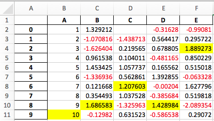
Export to LaTeX

There is support (since version 1.3.0) to export Styler to LaTeX. The documentation for the .to_latex method gives further detail and numerous examples.

More About CSS and HTML

Cascading Style Sheet (CSS) language, which is designed to influence how a browser renders HTML elements, has its own peculiarities. It never reports errors: it just silently ignores them and doesn’t render your objects how you intend so can sometimes be frustrating. Here is a very brief primer on how Styler creates HTML and interacts with CSS, with advice on common pitfalls to avoid.

CSS Classes and Ids

The precise structure of the CSS class attached to each cell is as follows.

• Cells with Index and Column names include index_name and level<k> where k is its level in a MultiIndex

• Index label cells include

  • row_heading

  • level<k> where k is the level in a MultiIndex

  • row<m> where m is the numeric position of the row

• Column label cells include

  • col_heading

  • level<k> where k is the level in a MultiIndex

  • col<n> where n is the numeric position of the column

• Data cells include

  • data

  • row<m>, where m is the numeric position of the cell.

  • col<n>, where n is the numeric position of the cell.

• Blank cells include blank

• Trimmed cells include col_trim or row_trim

The structure of the id is T_uuid_level<k>_row<m>_col<n> where level<k> is used only on headings, and headings will only have either row<m> or col<n> whichever is needed. By default we’ve also prepended each row/column identifier with a UUID unique to each DataFrame so that the style from one doesn’t collide with the styling from another within the same notebook or page. You can read more about the use of UUIDs in Optimization.

We can see example of the HTML by calling the .to_html() method.

print(
    pd.DataFrame(
        [[1, 2], [3, 4]], index=["i1", "i2"], columns=["c1", "c2"]
    ).style.to_html()
)

<style type="text/css">
</style>
<table id="T_649ed">
  <thead>
    <tr>
      <th class="blank level0" >&nbsp;</th>
      <th id="T_649ed_level0_col0" class="col_heading level0 col0" >c1</th>
      <th id="T_649ed_level0_col1" class="col_heading level0 col1" >c2</th>
    </tr>
  </thead>
  <tbody>
    <tr>
      <th id="T_649ed_level0_row0" class="row_heading level0 row0" >i1</th>
      <td id="T_649ed_row0_col0" class="data row0 col0" >1</td>
      <td id="T_649ed_row0_col1" class="data row0 col1" >2</td>
    </tr>
    <tr>
      <th id="T_649ed_level0_row1" class="row_heading level0 row1" >i2</th>
      <td id="T_649ed_row1_col0" class="data row1 col0" >3</td>
      <td id="T_649ed_row1_col1" class="data row1 col1" >4</td>
    </tr>
  </tbody>
</table>

CSS Hierarchies

The examples have shown that when CSS styles overlap, the one that comes last in the HTML render, takes precedence. So the following yield different results:

df4 = pd.DataFrame([["text"]])
df4.style.map(lambda x: "color:green;").map(lambda x: "color:red;")

	0
0	text

df4.style.map(lambda x: "color:red;").map(lambda x: "color:green;")

	0
0	text

This is only true for CSS rules that are equivalent in hierarchy, or importance. You can read more about CSS specificity here but for our purposes it suffices to summarize the key points:

A CSS importance score for each HTML element is derived by starting at zero and adding:

• 1000 for an inline style attribute

• 100 for each ID

• 10 for each attribute, class or pseudo-class

• 1 for each element name or pseudo-element

Let’s use this to describe the action of the following configurations

df4.style.set_uuid("a_").set_table_styles(
    [{"selector": "td", "props": "color:red;"}]
).map(lambda x: "color:green;")

	0
0	text

This text is red because the generated selector #T_a_ td is worth 101 (ID plus element), whereas #T_a_row0_col0 is only worth 100 (ID), so is considered inferior even though in the HTML it comes after the previous.

df4.style.set_uuid("b_").set_table_styles(
    [
        {"selector": "td", "props": "color:red;"},
        {"selector": ".cls-1", "props": "color:blue;"},
    ]
).map(lambda x: "color:green;").set_td_classes(pd.DataFrame([["cls-1"]]))

	0
0	text

In the above case the text is blue because the selector #T_b_ .cls-1 is worth 110 (ID plus class), which takes precedence.

df4.style.set_uuid("c_").set_table_styles(
    [
        {"selector": "td", "props": "color:red;"},
        {"selector": ".cls-1", "props": "color:blue;"},
        {"selector": "td.data", "props": "color:yellow;"},
    ]
).map(lambda x: "color:green;").set_td_classes(pd.DataFrame([["cls-1"]]))

	0
0	text

Now we have created another table style this time the selector T_c_ td.data (ID plus element plus class) gets bumped up to 111.

If your style fails to be applied, and its really frustrating, try the !important trump card.

df4.style.set_uuid("d_").set_table_styles(
    [
        {"selector": "td", "props": "color:red;"},
        {"selector": ".cls-1", "props": "color:blue;"},
        {"selector": "td.data", "props": "color:yellow;"},
    ]
).map(lambda x: "color:green !important;").set_td_classes(pd.DataFrame([["cls-1"]]))

	0
0	text

Finally got that green text after all!

Extensibility

The core of pandas is, and will remain, its “high-performance, easy-to-use data structures”. With that in mind, we hope that DataFrame.style accomplishes two goals

• Provide an API that is pleasing to use interactively and is “good enough” for many tasks

• Provide the foundations for dedicated libraries to build on

If you build a great library on top of this, let us know and we’ll link to it.

Subclassing

If the default template doesn’t quite suit your needs, you can subclass Styler and extend or override the template. We’ll show an example of extending the default template to insert a custom header before each table.

from jinja2 import Environment, ChoiceLoader, FileSystemLoader
from IPython.display import HTML
from pandas.io.formats.style import Styler

We’ll use the following template:

with open("templates/myhtml.tpl") as f_html:
    print(f_html.read())

{% extends "html_table.tpl" %}
{% block table %}
<h1>{{ table_title|default("My Table") }}</h1>
{{ super() }}
{% endblock table %}

Now that we’ve created a template, we need to set up a subclass of Styler that knows about it.

class MyStyler(Styler):
    env = Environment(
        loader=ChoiceLoader(
            [
                FileSystemLoader("templates"),  # contains ours
                Styler.loader,  # the default
            ]
        )
    )
    template_html_table = env.get_template("myhtml.tpl")

Notice that we include the original loader in our environment’s loader. That’s because we extend the original template, so the Jinja environment needs to be able to find it.

Now we can use that custom styler. It’s __init__ takes a DataFrame.

MyStyler(df3)

My Table

		c1	c2	c3	c4
A	r1	1.322000	-1.853666	-0.159457	1.635827
	r2	1.069083	-0.301842	-0.507852	0.411485
B	r1	-0.120062	0.119718	-0.028951	1.083671
	r2	-1.093112	-0.537696	-1.488655	-0.175511

Our custom template accepts a table_title keyword. We can provide the value in the .to_html method.

HTML(MyStyler(df3).to_html(table_title="Extending Example"))

Extending Example

		c1	c2	c3	c4
A	r1	1.322000	-1.853666	-0.159457	1.635827
	r2	1.069083	-0.301842	-0.507852	0.411485
B	r1	-0.120062	0.119718	-0.028951	1.083671
	r2	-1.093112	-0.537696	-1.488655	-0.175511

For convenience, we provide the Styler.from_custom_template method that does the same as the custom subclass.

EasyStyler = Styler.from_custom_template("templates", "myhtml.tpl")
HTML(EasyStyler(df3).to_html(table_title="Another Title"))

Another Title

		c1	c2	c3	c4
A	r1	1.322000	-1.853666	-0.159457	1.635827
	r2	1.069083	-0.301842	-0.507852	0.411485
B	r1	-0.120062	0.119718	-0.028951	1.083671
	r2	-1.093112	-0.537696	-1.488655	-0.175511

Template Structure

Here’s the template structure for the both the style generation template and the table generation template:

Style template:

HTML(style_structure)

before_style

style

<style type="text/css">

table_styles

before_cellstyle

cellstyle

</style>

Table template:

HTML(table_structure)

before_table

table

<table ...>

caption

thead

before_head_rows

head_tr (loop over headers)

after_head_rows

tbody

before_rows

tr (loop over data rows)

after_rows

</table>

after_table

See the template in the GitHub repo for more details.