Indexing and Selecting Data
The axis labeling information in pandas objects serves many purposes:
- Identifies data (i.e. provides metadata) using known indicators, important for analysis, visualization, and interactive console display
- Enables automatic and explicit data alignment
- Allows intuitive getting and setting of subsets of the data set
In this section, we will focus on the final point: namely, how to slice, dice, and generally get and set subsets of pandas objects. The primary focus will be on Series and DataFrame as they have received more development attention in this area. Expect more work to be invested higher-dimensional data structures (including Panel) in the future, especially in label-based advanced indexing.
Note
The Python and NumPy indexing operators [] and attribute operator . provide quick and easy access to pandas data structures across a wide range of use cases. This makes interactive work intuitive, as there’s little new to learn if you already know how to deal with Python dictionaries and NumPy arrays. However, since the type of the data to be accessed isn’t known in advance, directly using standard operators has some optimization limits. For production code, we recommended that you take advantage of the optimized pandas data access methods exposed in this chapter.
Warning
Whether a copy or a reference is returned for a setting operation, may depend on the context. This is sometimes called chained assignment and should be avoided. See Returning a View versus Copy
See the cookbook for some advanced strategies
Different Choices for Indexing (loc, iloc, and ix)
New in version 0.11.0.
Object selection has had a number of user-requested additions in order to support more explicit location based indexing. pandas now supports three types of multi-axis indexing.
.loc is strictly label based, will raise KeyError when the items are not found, allowed inputs are:
- A single label, e.g. 5 or 'a', (note that 5 is interpreted as a label of the index. This use is not an integer position along the index)
- A list or array of labels ['a', 'b', 'c']
- A slice object with labels 'a':'f', (note that contrary to usual python slices, both the start and the stop are included!)
- A boolean array
See more at Selection by Label
.iloc is strictly integer position based (from 0 to length-1 of the axis), will raise IndexError if an indexer is requested and it is out-of-bounds, except slice indexers which allow out-of-bounds indexing. (this conforms with python/numpy slice semantics). Allowed inputs are:
- An integer e.g. 5
- A list or array of integers [4, 3, 0]
- A slice object with ints 1:7
See more at Selection by Position
.ix supports mixed integer and label based access. It is primarily label based, but will fallback to integer positional access. .ix is the most general and will support any of the inputs to .loc and .iloc, as well as support for floating point label schemes. .ix is especially useful when dealing with mixed positional and label based hierarchial indexes. As using integer slices with .ix have different behavior depending on whether the slice is interpreted as position based or label based, it’s usually better to be explicit and use .iloc or .loc.
See more at Advanced Indexing, Advanced Hierarchical and Fallback Indexing
Getting values from an object with multi-axes selection uses the following notation (using .loc as an example, but applies to .iloc and .ix as well). Any of the axes accessors may be the null slice :. Axes left out of the specification are assumed to be :. (e.g. p.loc['a'] is equiv to p.loc['a', :, :])
| Object Type | Indexers |
|---|---|
| Series | s.loc[indexer] |
| DataFrame | df.loc[row_indexer,column_indexer] |
| Panel | p.loc[item_indexer,major_indexer,minor_indexer] |
Deprecations
Beginning with version 0.11.0, it’s recommended that you transition away from the following methods as they may be deprecated in future versions.
- irow
- icol
- iget_value
See the section Selection by Position for substitutes.
Basics
As mentioned when introducing the data structures in the last section, the primary function of indexing with [] (a.k.a. __getitem__ for those familiar with implementing class behavior in Python) is selecting out lower-dimensional slices. Thus,
| Object Type | Selection | Return Value Type |
|---|---|---|
| Series | series[label] | scalar value |
| DataFrame | frame[colname] | Series corresponding to colname |
| Panel | panel[itemname] | DataFrame corresponing to the itemname |
Here we construct a simple time series data set to use for illustrating the indexing functionality:
In [1]: dates = date_range('1/1/2000', periods=8)

In [2]: df = DataFrame(randn(8, 4), index=dates, columns=['A', 'B', 'C', 'D'])

In [3]: df
Out[3]:
                   A         B         C         D
2000-01-01  0.469112 -0.282863 -1.509059 -1.135632
2000-01-02  1.212112 -0.173215  0.119209 -1.044236
2000-01-03 -0.861849 -2.104569 -0.494929  1.071804
2000-01-04  0.721555 -0.706771 -1.039575  0.271860
2000-01-05 -0.424972  0.567020  0.276232 -1.087401
2000-01-06 -0.673690  0.113648 -1.478427  0.524988
2000-01-07  0.404705  0.577046 -1.715002 -1.039268
2000-01-08 -0.370647 -1.157892 -1.344312  0.844885

In [4]: panel = Panel({'one' : df, 'two' : df - df.mean()})

In [5]: panel
Out[5]:
<class 'pandas.core.panel.Panel'>
Dimensions: 2 (items) x 8 (major_axis) x 4 (minor_axis)
Items axis: one to two
Major_axis axis: 2000-01-01 00:00:00 to 2000-01-08 00:00:00
Minor_axis axis: A to D
Note
None of the indexing functionality is time series specific unless specifically stated.
Thus, as per above, we have the most basic indexing using []:
In [6]: s = df['A']

In [7]: s[dates[5]]
Out[7]: -0.67368970808837025

In [8]: panel['two']
Out[8]:
                   A         B         C         D
2000-01-01  0.409571  0.113086 -0.610826 -0.936507
2000-01-02  1.152571  0.222735  1.017442 -0.845111
2000-01-03 -0.921390 -1.708620  0.403304  1.270929
2000-01-04  0.662014 -0.310822 -0.141342  0.470985
2000-01-05 -0.484513  0.962970  1.174465 -0.888276
2000-01-06 -0.733231  0.509598 -0.580194  0.724113
2000-01-07  0.345164  0.972995 -0.816769 -0.840143
2000-01-08 -0.430188 -0.761943 -0.446079  1.044010
You can pass a list of columns to [] to select columns in that order. If a column is not contained in the DataFrame, an exception will be raised. Multiple columns can also be set in this manner:
In [9]: df
Out[9]:
                   A         B         C         D
2000-01-01  0.469112 -0.282863 -1.509059 -1.135632
2000-01-02  1.212112 -0.173215  0.119209 -1.044236
2000-01-03 -0.861849 -2.104569 -0.494929  1.071804
2000-01-04  0.721555 -0.706771 -1.039575  0.271860
2000-01-05 -0.424972  0.567020  0.276232 -1.087401
2000-01-06 -0.673690  0.113648 -1.478427  0.524988
2000-01-07  0.404705  0.577046 -1.715002 -1.039268
2000-01-08 -0.370647 -1.157892 -1.344312  0.844885

In [10]: df[['B', 'A']] = df[['A', 'B']]

In [11]: df
Out[11]:
                   A         B         C         D
2000-01-01 -0.282863  0.469112 -1.509059 -1.135632
2000-01-02 -0.173215  1.212112  0.119209 -1.044236
2000-01-03 -2.104569 -0.861849 -0.494929  1.071804
2000-01-04 -0.706771  0.721555 -1.039575  0.271860
2000-01-05  0.567020 -0.424972  0.276232 -1.087401
2000-01-06  0.113648 -0.673690 -1.478427  0.524988
2000-01-07  0.577046  0.404705 -1.715002 -1.039268
2000-01-08 -1.157892 -0.370647 -1.344312  0.844885
You may find this useful for applying a transform (in-place) to a subset of the columns.
Attribute Access
You may access an index on a Series, column on a DataFrame, and a item on a Panel directly as an attribute:
In [12]: sa = Series([1,2,3],index=list('abc'))

In [13]: dfa = df.copy()
In [14]: sa.b
Out[14]: 2

In [15]: dfa.A
Out[15]:
2000-01-01   -0.282863
2000-01-02   -0.173215
2000-01-03   -2.104569
2000-01-04   -0.706771
2000-01-05    0.567020
2000-01-06    0.113648
2000-01-07    0.577046
2000-01-08   -1.157892
Freq: D, Name: A, dtype: float64

In [16]: panel.one
Out[16]:
                   A         B         C         D
2000-01-01  0.469112 -0.282863 -1.509059 -1.135632
2000-01-02  1.212112 -0.173215  0.119209 -1.044236
2000-01-03 -0.861849 -2.104569 -0.494929  1.071804
2000-01-04  0.721555 -0.706771 -1.039575  0.271860
2000-01-05 -0.424972  0.567020  0.276232 -1.087401
2000-01-06 -0.673690  0.113648 -1.478427  0.524988
2000-01-07  0.404705  0.577046 -1.715002 -1.039268
2000-01-08 -0.370647 -1.157892 -1.344312  0.844885
You can use attribute access to modify an existing element of a Series or column of a DataFrame, but be careful; if you try to use attribute access to create a new column, it fails silently, creating a new attribute rather than a new column.
In [17]: sa.a = 5

In [18]: sa
Out[18]:
a    5
b    2
c    3
dtype: int64

In [19]: dfa.A = list(range(len(dfa.index)))       # ok if A already exists

In [20]: dfa
Out[20]:
            A         B         C         D
2000-01-01  0  0.469112 -1.509059 -1.135632
2000-01-02  1  1.212112  0.119209 -1.044236
2000-01-03  2 -0.861849 -0.494929  1.071804
2000-01-04  3  0.721555 -1.039575  0.271860
2000-01-05  4 -0.424972  0.276232 -1.087401
2000-01-06  5 -0.673690 -1.478427  0.524988
2000-01-07  6  0.404705 -1.715002 -1.039268
2000-01-08  7 -0.370647 -1.344312  0.844885

In [21]: dfa['A'] = list(range(len(dfa.index)))    # use this form to create a new column

In [22]: dfa
Out[22]:
            A         B         C         D
2000-01-01  0  0.469112 -1.509059 -1.135632
2000-01-02  1  1.212112  0.119209 -1.044236
2000-01-03  2 -0.861849 -0.494929  1.071804
2000-01-04  3  0.721555 -1.039575  0.271860
2000-01-05  4 -0.424972  0.276232 -1.087401
2000-01-06  5 -0.673690 -1.478427  0.524988
2000-01-07  6  0.404705 -1.715002 -1.039268
2000-01-08  7 -0.370647 -1.344312  0.844885
Warning
- You can use this access only if the index element is a valid python identifier, e.g. s.1 is not allowed. see here for an explanation of valid identifiers.
- The attribute will not be available if it conflicts with an existing method name, e.g. s.min is not allowed.
- The Series/Panel accesses are available starting in 0.13.0.
If you are using the IPython environment, you may also use tab-completion to see these accessable attributes.
Slicing ranges
The most robust and consistent way of slicing ranges along arbitrary axes is described in the Selection by Position section detailing the .iloc method. For now, we explain the semantics of slicing using the [] operator.
With Series, the syntax works exactly as with an ndarray, returning a slice of the values and the corresponding labels:
In [23]: s[:5]
Out[23]:
2000-01-01   -0.282863
2000-01-02   -0.173215
2000-01-03   -2.104569
2000-01-04   -0.706771
2000-01-05    0.567020
Freq: D, Name: A, dtype: float64

In [24]: s[::2]
Out[24]:
2000-01-01   -0.282863
2000-01-03   -2.104569
2000-01-05    0.567020
2000-01-07    0.577046
Freq: 2D, Name: A, dtype: float64

In [25]: s[::-1]
Out[25]:
2000-01-08   -1.157892
2000-01-07    0.577046
2000-01-06    0.113648
2000-01-05    0.567020
2000-01-04   -0.706771
2000-01-03   -2.104569
2000-01-02   -0.173215
2000-01-01   -0.282863
Freq: -1D, Name: A, dtype: float64
Note that setting works as well:
In [26]: s2 = s.copy()

In [27]: s2[:5] = 0

In [28]: s2
Out[28]:
2000-01-01    0.000000
2000-01-02    0.000000
2000-01-03    0.000000
2000-01-04    0.000000
2000-01-05    0.000000
2000-01-06    0.113648
2000-01-07    0.577046
2000-01-08   -1.157892
Freq: D, Name: A, dtype: float64
With DataFrame, slicing inside of [] slices the rows. This is provided largely as a convenience since it is such a common operation.
In [29]: df[:3]
Out[29]:
                   A         B         C         D
2000-01-01 -0.282863  0.469112 -1.509059 -1.135632
2000-01-02 -0.173215  1.212112  0.119209 -1.044236
2000-01-03 -2.104569 -0.861849 -0.494929  1.071804

In [30]: df[::-1]
Out[30]:
                   A         B         C         D
2000-01-08 -1.157892 -0.370647 -1.344312  0.844885
2000-01-07  0.577046  0.404705 -1.715002 -1.039268
2000-01-06  0.113648 -0.673690 -1.478427  0.524988
2000-01-05  0.567020 -0.424972  0.276232 -1.087401
2000-01-04 -0.706771  0.721555 -1.039575  0.271860
2000-01-03 -2.104569 -0.861849 -0.494929  1.071804
2000-01-02 -0.173215  1.212112  0.119209 -1.044236
2000-01-01 -0.282863  0.469112 -1.509059 -1.135632
Selection By Label
Warning
Whether a copy or a reference is returned for a setting operation, may depend on the context. This is sometimes called chained assignment and should be avoided. See Returning a View versus Copy
pandas provides a suite of methods in order to have purely label based indexing. This is a strict inclusion based protocol. ALL of the labels for which you ask, must be in the index or a KeyError will be raised! When slicing, the start bound is included, AND the stop bound is included. Integers are valid labels, but they refer to the label and not the position.
The .loc attribute is the primary access method. The following are valid inputs:
- A single label, e.g. 5 or 'a', (note that 5 is interpreted as a label of the index. This use is not an integer position along the index)
- A list or array of labels ['a', 'b', 'c']
- A slice object with labels 'a':'f' (note that contrary to usual python slices, both the start and the stop are included!)
- A boolean array
In [31]: s1 = Series(np.random.randn(6),index=list('abcdef'))

In [32]: s1
Out[32]:
a    1.075770
b   -0.109050
c    1.643563
d   -1.469388
e    0.357021
f   -0.674600
dtype: float64

In [33]: s1.loc['c':]
Out[33]:
c    1.643563
d   -1.469388
e    0.357021
f   -0.674600
dtype: float64

In [34]: s1.loc['b']
Out[34]: -0.10904997528022223
Note that setting works as well:
In [35]: s1.loc['c':] = 0

In [36]: s1
Out[36]:
a    1.07577
b   -0.10905
c    0.00000
d    0.00000
e    0.00000
f    0.00000
dtype: float64
With a DataFrame
In [37]: df1 = DataFrame(np.random.randn(6,4),
   ....:                 index=list('abcdef'),
   ....:                 columns=list('ABCD'))
   ....:

In [38]: df1
Out[38]:
          A         B         C         D
a -1.776904 -0.968914 -1.294524  0.413738
b  0.276662 -0.472035 -0.013960 -0.362543
c -0.006154 -0.923061  0.895717  0.805244
d -1.206412  2.565646  1.431256  1.340309
e -1.170299 -0.226169  0.410835  0.813850
f  0.132003 -0.827317 -0.076467 -1.187678

In [39]: df1.loc[['a','b','d'],:]
Out[39]:
          A         B         C         D
a -1.776904 -0.968914 -1.294524  0.413738
b  0.276662 -0.472035 -0.013960 -0.362543
d -1.206412  2.565646  1.431256  1.340309
Accessing via label slices
In [40]: df1.loc['d':,'A':'C']
Out[40]:
          A         B         C
d -1.206412  2.565646  1.431256
e -1.170299 -0.226169  0.410835
f  0.132003 -0.827317 -0.076467
For getting a cross section using a label (equiv to df.xs('a'))
In [41]: df1.loc['a']
Out[41]:
A   -1.776904
B   -0.968914
C   -1.294524
D    0.413738
Name: a, dtype: float64
For getting values with a boolean array
In [42]: df1.loc['a']>0
Out[42]:
A    False
B    False
C    False
D     True
Name: a, dtype: bool

In [43]: df1.loc[:,df1.loc['a']>0]
Out[43]:
          D
a  0.413738
b -0.362543
c  0.805244
d  1.340309
e  0.813850
f -1.187678
For getting a value explicity (equiv to deprecated df.get_value('a','A'))
# this is also equivalent to ``df1.at['a','A']``
In [44]: df1.loc['a','A']
Out[44]: -1.7769037169718671
Selection By Position
Warning
Whether a copy or a reference is returned for a setting operation, may depend on the context. This is sometimes called chained assignment and should be avoided. See Returning a View versus Copy
pandas provides a suite of methods in order to get purely integer based indexing. The semantics follow closely python and numpy slicing. These are 0-based indexing. When slicing, the start bounds is included, while the upper bound is excluded. Trying to use a non-integer, even a valid label will raise a IndexError.
The .iloc attribute is the primary access method. The following are valid inputs:
- An integer e.g. 5
- A list or array of integers [4, 3, 0]
- A slice object with ints 1:7
In [45]: s1 = Series(np.random.randn(5),index=list(range(0,10,2)))

In [46]: s1
Out[46]:
0    1.130127
2   -1.436737
4   -1.413681
6    1.607920
8    1.024180
dtype: float64

In [47]: s1.iloc[:3]
Out[47]:
0    1.130127
2   -1.436737
4   -1.413681
dtype: float64

In [48]: s1.iloc[3]
Out[48]: 1.6079204745847746
Note that setting works as well:
In [49]: s1.iloc[:3] = 0

In [50]: s1
Out[50]:
0    0.00000
2    0.00000
4    0.00000
6    1.60792
8    1.02418
dtype: float64
With a DataFrame
In [51]: df1 = DataFrame(np.random.randn(6,4),
   ....:                 index=list(range(0,12,2)),
   ....:                 columns=list(range(0,8,2)))
   ....:

In [52]: df1
Out[52]:
           0         2         4         6
0   0.569605  0.875906 -2.211372  0.974466
2  -2.006747 -0.410001 -0.078638  0.545952
4  -1.219217 -1.226825  0.769804 -1.281247
6  -0.727707 -0.121306 -0.097883  0.695775
8   0.341734  0.959726 -1.110336 -0.619976
10  0.149748 -0.732339  0.687738  0.176444
Select via integer slicing
In [53]: df1.iloc[:3]
Out[53]:
          0         2         4         6
0  0.569605  0.875906 -2.211372  0.974466
2 -2.006747 -0.410001 -0.078638  0.545952
4 -1.219217 -1.226825  0.769804 -1.281247

In [54]: df1.iloc[1:5,2:4]
Out[54]:
          4         6
2 -0.078638  0.545952
4  0.769804 -1.281247
6 -0.097883  0.695775
8 -1.110336 -0.619976
Select via integer list
In [55]: df1.iloc[[1,3,5],[1,3]]
Out[55]:
           2         6
2  -0.410001  0.545952
6  -0.121306  0.695775
10 -0.732339  0.176444
For slicing rows explicitly (equiv to deprecated df.irow(slice(1,3))).
In [56]: df1.iloc[1:3,:]
Out[56]:
          0         2         4         6
2 -2.006747 -0.410001 -0.078638  0.545952
4 -1.219217 -1.226825  0.769804 -1.281247
For slicing columns explicitly (equiv to deprecated df.icol(slice(1,3))).
In [57]: df1.iloc[:,1:3]
Out[57]:
           2         4
0   0.875906 -2.211372
2  -0.410001 -0.078638
4  -1.226825  0.769804
6  -0.121306 -0.097883
8   0.959726 -1.110336
10 -0.732339  0.687738
For getting a scalar via integer position (equiv to deprecated df.get_value(1,1))
# this is also equivalent to ``df1.iat[1,1]``
In [58]: df1.iloc[1,1]
Out[58]: -0.41000056806065832
For getting a cross section using an integer position (equiv to df.xs(1))
In [59]: df1.iloc[1]
Out[59]:
0   -2.006747
2   -0.410001
4   -0.078638
6    0.545952
Name: 2, dtype: float64
There is one signficant departure from standard python/numpy slicing semantics. python/numpy allow slicing past the end of an array without an associated error.
# these are allowed in python/numpy.
In [60]: x = list('abcdef')

In [61]: x[4:10]
Out[61]: ['e', 'f']

In [62]: x[8:10]
Out[62]: []
- as of v0.14.0, iloc will now accept out-of-bounds indexers for slices, e.g. a value that exceeds the length of the object being indexed. These will be excluded. This will make pandas conform more with pandas/numpy indexing of out-of-bounds values. A single indexer / list of indexers that is out-of-bounds will still raise IndexError (GH6296, GH6299). This could result in an empty axis (e.g. an empty DataFrame being returned)
In [63]: dfl = DataFrame(np.random.randn(5,2),columns=list('AB'))

In [64]: dfl
Out[64]:
          A         B
0  0.403310 -0.154951
1  0.301624 -2.179861
2 -1.369849 -0.954208
3  1.462696 -1.743161
4 -0.826591 -0.345352

In [65]: dfl.iloc[:,2:3]
Out[65]:
Empty DataFrame
Columns: []
Index: [0, 1, 2, 3, 4]

In [66]: dfl.iloc[:,1:3]
Out[66]:
          B
0 -0.154951
1 -2.179861
2 -0.954208
3 -1.743161
4 -0.345352

In [67]: dfl.iloc[4:6]
Out[67]:
          A         B
4 -0.826591 -0.345352
These are out-of-bounds selections
dfl.iloc[[4,5,6]]
IndexError: positional indexers are out-of-bounds

dfl.iloc[:,4]
IndexError: single positional indexer is out-of-bounds
Setting With Enlargement
New in version 0.13.
The .loc/.ix/[] operations can perform enlargement when setting a non-existant key for that axis.
In the Series case this is effectively an appending operation
In [68]: se = Series([1,2,3])

In [69]: se
Out[69]:
0    1
1    2
2    3
dtype: int64

In [70]: se[5] = 5.

In [71]: se
Out[71]:
0    1
1    2
2    3
5    5
dtype: float64
A DataFrame can be enlarged on either axis via .loc
In [72]: dfi = DataFrame(np.arange(6).reshape(3,2),
   ....:                 columns=['A','B'])
   ....:

In [73]: dfi
Out[73]:
   A  B
0  0  1
1  2  3
2  4  5

In [74]: dfi.loc[:,'C'] = dfi.loc[:,'A']

In [75]: dfi
Out[75]:
   A  B  C
0  0  1  0
1  2  3  2
2  4  5  4
This is like an append operation on the DataFrame.
In [76]: dfi.loc[3] = 5

In [77]: dfi
Out[77]:
   A  B  C
0  0  1  0
1  2  3  2
2  4  5  4
3  5  5  5
Fast scalar value getting and setting
Since indexing with [] must handle a lot of cases (single-label access, slicing, boolean indexing, etc.), it has a bit of overhead in order to figure out what you’re asking for. If you only want to access a scalar value, the fastest way is to use the at and iat methods, which are implemented on all of the data structures.
Similary to loc, at provides label based scalar lookups, while, iat provides integer based lookups analagously to iloc
In [78]: s.iat[5]
Out[78]: 0.11364840968888545

In [79]: df.at[dates[5], 'A']
Out[79]: 0.11364840968888545

In [80]: df.iat[3, 0]
Out[80]: -0.70677113363008448
You can also set using these same indexers.
In [81]: df.at[dates[5], 'E'] = 7

In [82]: df.iat[3, 0] = 7
at may enlarge the object in-place as above if the indexer is missing.
In [83]: df.at[dates[-1]+1, 0] = 7

In [84]: df
Out[84]:
                   A         B         C         D   E   0
2000-01-01 -0.282863  0.469112 -1.509059 -1.135632 NaN NaN
2000-01-02 -0.173215  1.212112  0.119209 -1.044236 NaN NaN
2000-01-03 -2.104569 -0.861849 -0.494929  1.071804 NaN NaN
2000-01-04  7.000000  0.721555 -1.039575  0.271860 NaN NaN
2000-01-05  0.567020 -0.424972  0.276232 -1.087401 NaN NaN
2000-01-06  0.113648 -0.673690 -1.478427  0.524988   7 NaN
2000-01-07  0.577046  0.404705 -1.715002 -1.039268 NaN NaN
2000-01-08 -1.157892 -0.370647 -1.344312  0.844885 NaN NaN
2000-01-09       NaN       NaN       NaN       NaN NaN   7
Boolean indexing
Another common operation is the use of boolean vectors to filter the data. The operators are: | for or, & for and, and ~ for not. These must be grouped by using parentheses.
Using a boolean vector to index a Series works exactly as in a numpy ndarray:
In [85]: s[s > 0]
Out[85]:
2000-01-05    0.567020
2000-01-06    0.113648
2000-01-07    0.577046
Freq: D, Name: A, dtype: float64

In [86]: s[(s < 0) & (s > -0.5)]
Out[86]:
2000-01-01   -0.282863
2000-01-02   -0.173215
Freq: D, Name: A, dtype: float64

In [87]: s[(s < -1) | (s > 1 )]
Out[87]:
2000-01-03   -2.104569
2000-01-08   -1.157892
Name: A, dtype: float64

In [88]: s[~(s < 0)]
Out[88]:
2000-01-05    0.567020
2000-01-06    0.113648
2000-01-07    0.577046
Freq: D, Name: A, dtype: float64
You may select rows from a DataFrame using a boolean vector the same length as the DataFrame’s index (for example, something derived from one of the columns of the DataFrame):
In [89]: df[df['A'] > 0]
Out[89]:
                   A         B         C         D   E   0
2000-01-04  7.000000  0.721555 -1.039575  0.271860 NaN NaN
2000-01-05  0.567020 -0.424972  0.276232 -1.087401 NaN NaN
2000-01-06  0.113648 -0.673690 -1.478427  0.524988   7 NaN
2000-01-07  0.577046  0.404705 -1.715002 -1.039268 NaN NaN
List comprehensions and map method of Series can also be used to produce more complex criteria:
In [90]: df2 = DataFrame({'a' : ['one', 'one', 'two', 'three', 'two', 'one', 'six'],
   ....:                  'b' : ['x', 'y', 'y', 'x', 'y', 'x', 'x'],
   ....:                  'c' : randn(7)})
   ....:

# only want 'two' or 'three'
In [91]: criterion = df2['a'].map(lambda x: x.startswith('t'))

In [92]: df2[criterion]
Out[92]:
       a  b         c
2    two  y  0.995761
3  three  x  2.396780
4    two  y  0.014871

# equivalent but slower
In [93]: df2[[x.startswith('t') for x in df2['a']]]
Out[93]:
       a  b         c
2    two  y  0.995761
3  three  x  2.396780
4    two  y  0.014871

# Multiple criteria
In [94]: df2[criterion & (df2['b'] == 'x')]
Out[94]:
       a  b        c
3  three  x  2.39678
Note, with the choice methods Selection by Label, Selection by Position, and Advanced Indexing you may select along more than one axis using boolean vectors combined with other indexing expressions.
In [95]: df2.loc[criterion & (df2['b'] == 'x'),'b':'c']
Out[95]:
   b        c
3  x  2.39678
Indexing with isin
Consider the isin method of Series, which returns a boolean vector that is true wherever the Series elements exist in the passed list. This allows you to select rows where one or more columns have values you want:
In [96]: s = Series(np.arange(5),index=np.arange(5)[::-1],dtype='int64')

In [97]: s
Out[97]:
4    0
3    1
2    2
1    3
0    4
dtype: int64

In [98]: s.isin([2, 4])
Out[98]:
4    False
3    False
2     True
1    False
0     True
dtype: bool

In [99]: s[s.isin([2, 4])]
Out[99]:
2    2
0    4
dtype: int64
DataFrame also has an isin method. When calling isin, pass a set of values as either an array or dict. If values is an array, isin returns a DataFrame of booleans that is the same shape as the original DataFrame, with True wherever the element is in the sequence of values.
In [100]: df = DataFrame({'vals': [1, 2, 3, 4], 'ids': ['a', 'b', 'f', 'n'],
   .....:                 'ids2': ['a', 'n', 'c', 'n']})
   .....:

In [101]: values = ['a', 'b', 1, 3]

In [102]: df.isin(values)
Out[102]:
     ids   ids2   vals
0   True   True   True
1   True  False  False
2  False  False   True
3  False  False  False
Oftentimes you’ll want to match certain values with certain columns. Just make values a dict where the key is the column, and the value is a list of items you want to check for.
In [103]: values = {'ids': ['a', 'b'], 'vals': [1, 3]}

In [104]: df.isin(values)
Out[104]:
     ids   ids2   vals
0   True  False   True
1   True  False  False
2  False  False   True
3  False  False  False
Combine DataFrame’s isin with the any() and all() methods to quickly select subsets of your data that meet a given criteria. To select a row where each column meets its own criterion:
In [105]: values = {'ids': ['a', 'b'], 'ids2': ['a', 'c'], 'vals': [1, 3]}

In [106]: row_mask = df.isin(values).all(1)

In [107]: df[row_mask]
Out[107]:
  ids ids2  vals
0   a    a     1
The where() Method and Masking
Selecting values from a Series with a boolean vector generally returns a subset of the data. To guarantee that selection output has the same shape as the original data, you can use the where method in Series and DataFrame.
To return only the selected rows
In [108]: s[s > 0]
Out[108]:
3    1
2    2
1    3
0    4
dtype: int64
To return a Series of the same shape as the original
In [109]: s.where(s > 0)
Out[109]:
4   NaN
3     1
2     2
1     3
0     4
dtype: float64
Selecting values from a DataFrame with a boolean critierion now also preserves input data shape. where is used under the hood as the implementation. Equivalent is df.where(df < 0)
In [110]: df[df < 0]
Out[110]:
                   A         B         C         D
2000-01-01 -1.236269       NaN -0.487602 -0.082240
2000-01-02 -2.182937       NaN       NaN       NaN
2000-01-03       NaN -0.493662       NaN       NaN
2000-01-04       NaN -0.023688       NaN       NaN
2000-01-05       NaN -0.251905 -2.213588       NaN
2000-01-06       NaN       NaN -0.863838       NaN
2000-01-07 -1.048089 -0.025747 -0.988387       NaN
2000-01-08       NaN       NaN       NaN -0.055758
In addition, where takes an optional other argument for replacement of values where the condition is False, in the returned copy.
In [111]: df.where(df < 0, -df)
Out[111]:
                   A         B         C         D
2000-01-01 -1.236269 -0.896171 -0.487602 -0.082240
2000-01-02 -2.182937 -0.380396 -0.084844 -0.432390
2000-01-03 -1.519970 -0.493662 -0.600178 -0.274230
2000-01-04 -0.132885 -0.023688 -2.410179 -1.450520
2000-01-05 -0.206053 -0.251905 -2.213588 -1.063327
2000-01-06 -1.266143 -0.299368 -0.863838 -0.408204
2000-01-07 -1.048089 -0.025747 -0.988387 -0.094055
2000-01-08 -1.262731 -1.289997 -0.082423 -0.055758
You may wish to set values based on some boolean criteria. This can be done intuitively like so:
In [112]: s2 = s.copy()

In [113]: s2[s2 < 0] = 0

In [114]: s2
Out[114]:
4    0
3    1
2    2
1    3
0    4
dtype: int64

In [115]: df2 = df.copy()

In [116]: df2[df2 < 0] = 0

In [117]: df2
Out[117]:
                   A         B         C         D
2000-01-01  0.000000  0.896171  0.000000  0.000000
2000-01-02  0.000000  0.380396  0.084844  0.432390
2000-01-03  1.519970  0.000000  0.600178  0.274230
2000-01-04  0.132885  0.000000  2.410179  1.450520
2000-01-05  0.206053  0.000000  0.000000  1.063327
2000-01-06  1.266143  0.299368  0.000000  0.408204
2000-01-07  0.000000  0.000000  0.000000  0.094055
2000-01-08  1.262731  1.289997  0.082423  0.000000
By default, where returns a modified copy of the data. There is an optional parameter inplace so that the original data can be modified without creating a copy:
In [118]: df_orig = df.copy()

In [119]: df_orig.where(df > 0, -df, inplace=True);

In [120]: df_orig
Out[120]:
                   A         B         C         D
2000-01-01  1.236269  0.896171  0.487602  0.082240
2000-01-02  2.182937  0.380396  0.084844  0.432390
2000-01-03  1.519970  0.493662  0.600178  0.274230
2000-01-04  0.132885  0.023688  2.410179  1.450520
2000-01-05  0.206053  0.251905  2.213588  1.063327
2000-01-06  1.266143  0.299368  0.863838  0.408204
2000-01-07  1.048089  0.025747  0.988387  0.094055
2000-01-08  1.262731  1.289997  0.082423  0.055758
alignment
Furthermore, where aligns the input boolean condition (ndarray or DataFrame), such that partial selection with setting is possible. This is analagous to partial setting via .ix (but on the contents rather than the axis labels)
In [121]: df2 = df.copy()

In [122]: df2[ df2[1:4] > 0 ] = 3

In [123]: df2
Out[123]:
                   A         B         C         D
2000-01-01 -1.236269  0.896171 -0.487602 -0.082240
2000-01-02 -2.182937  3.000000  3.000000  3.000000
2000-01-03  3.000000 -0.493662  3.000000  3.000000
2000-01-04  3.000000 -0.023688  3.000000  3.000000
2000-01-05  0.206053 -0.251905 -2.213588  1.063327
2000-01-06  1.266143  0.299368 -0.863838  0.408204
2000-01-07 -1.048089 -0.025747 -0.988387  0.094055
2000-01-08  1.262731  1.289997  0.082423 -0.055758
New in version 0.13.
Where can also accept axis and level parameters to align the input when performing the where.
In [124]: df2 = df.copy()

In [125]: df2.where(df2>0,df2['A'],axis='index')
Out[125]:
                   A         B         C         D
2000-01-01 -1.236269  0.896171 -1.236269 -1.236269
2000-01-02 -2.182937  0.380396  0.084844  0.432390
2000-01-03  1.519970  1.519970  0.600178  0.274230
2000-01-04  0.132885  0.132885  2.410179  1.450520
2000-01-05  0.206053  0.206053  0.206053  1.063327
2000-01-06  1.266143  0.299368  1.266143  0.408204
2000-01-07 -1.048089 -1.048089 -1.048089  0.094055
2000-01-08  1.262731  1.289997  0.082423  1.262731
This is equivalent (but faster than) the following.
In [126]: df2 = df.copy()

In [127]: df.apply(lambda x, y: x.where(x>0,y), y=df['A'])
Out[127]:
                   A         B         C         D
2000-01-01 -1.236269  0.896171 -1.236269 -1.236269
2000-01-02 -2.182937  0.380396  0.084844  0.432390
2000-01-03  1.519970  1.519970  0.600178  0.274230
2000-01-04  0.132885  0.132885  2.410179  1.450520
2000-01-05  0.206053  0.206053  0.206053  1.063327
2000-01-06  1.266143  0.299368  1.266143  0.408204
2000-01-07 -1.048089 -1.048089 -1.048089  0.094055
2000-01-08  1.262731  1.289997  0.082423  1.262731
mask
mask is the inverse boolean operation of where.
In [128]: s.mask(s >= 0)
Out[128]:
4   NaN
3   NaN
2   NaN
1   NaN
0   NaN
dtype: float64

In [129]: df.mask(df >= 0)
Out[129]:
                   A         B         C         D
2000-01-01 -1.236269       NaN -0.487602 -0.082240
2000-01-02 -2.182937       NaN       NaN       NaN
2000-01-03       NaN -0.493662       NaN       NaN
2000-01-04       NaN -0.023688       NaN       NaN
2000-01-05       NaN -0.251905 -2.213588       NaN
2000-01-06       NaN       NaN -0.863838       NaN
2000-01-07 -1.048089 -0.025747 -0.988387       NaN
2000-01-08       NaN       NaN       NaN -0.055758
The query() Method (Experimental)
New in version 0.13.
DataFrame objects have a query() method that allows selection using an expression.
You can get the value of the frame where column b has values between the values of columns a and c. For example:
In [130]: n = 10

In [131]: df = DataFrame(rand(n, 3), columns=list('abc'))

In [132]: df
Out[132]:
          a         b         c
0  0.191519  0.622109  0.437728
1  0.785359  0.779976  0.272593
2  0.276464  0.801872  0.958139
3  0.875933  0.357817  0.500995
4  0.683463  0.712702  0.370251
5  0.561196  0.503083  0.013768
6  0.772827  0.882641  0.364886
7  0.615396  0.075381  0.368824
8  0.933140  0.651378  0.397203
9  0.788730  0.316836  0.568099

# pure python
In [133]: df[(df.a < df.b) & (df.b < df.c)]
Out[133]:
          a         b         c
2  0.276464  0.801872  0.958139

# query
In [134]: df.query('(a < b) & (b < c)')
Out[134]:
          a         b         c
2  0.276464  0.801872  0.958139
Do the same thing but fallback on a named index if there is no column with the name a.
In [135]: df = DataFrame(randint(n / 2, size=(n, 2)), columns=list('bc'))

In [136]: df.index.name = 'a'

In [137]: df
Out[137]:
   b  c
a
0  2  3
1  4  1
2  4  0
3  4  1
4  1  4
5  1  4
6  0  1
7  0  0
8  4  0
9  4  2

In [138]: df.query('a < b and b < c')
Out[138]:
   b  c
a
0  2  3
If instead you don’t want to or cannot name your index, you can use the name index in your query expression:
In [139]: df = DataFrame(randint(n, size=(n, 2)), columns=list('bc'))

In [140]: df
Out[140]:
   b  c
0  3  1
1  2  5
2  2  5
3  6  7
4  4  3
5  5  6
6  4  6
7  2  4
8  2  7
9  9  7

In [141]: df.query('index < b < c')
Out[141]:
   b  c
1  2  5
3  6  7
Note
If the name of your index overlaps with a column name, the column name is given precedence. For example,
In [142]: df = DataFrame({'a': randint(5, size=5)})

In [143]: df.index.name = 'a'

In [144]: df.query('a > 2') # uses the column 'a', not the index
Out[144]:
   a
a
0  3
3  4
You can still use the index in a query expression by using the special identifier ‘index’:
In [145]: df.query('index > 2')
Out[145]:
   a
a
3  4
4  1
If for some reason you have a column named index, then you can refer to the index as ilevel_0 as well, but at this point you should consider renaming your columns to something less ambiguous.
MultiIndex query() Syntax
You can also use the levels of a DataFrame with a MultiIndex as if they were columns in the frame:
In [146]: import pandas.util.testing as tm

In [147]: n = 10

In [148]: colors = tm.choice(['red', 'green'], size=n)

In [149]: foods = tm.choice(['eggs', 'ham'], size=n)

In [150]: colors
Out[150]:
array(['red', 'green', 'red', 'green', 'red', 'green', 'red', 'green',
       'green', 'green'],
      dtype='|S5')

In [151]: foods
Out[151]:
array(['ham', 'eggs', 'ham', 'ham', 'ham', 'eggs', 'eggs', 'eggs', 'ham',
       'eggs'],
      dtype='|S4')

In [152]: index = MultiIndex.from_arrays([colors, foods], names=['color', 'food'])

In [153]: df = DataFrame(randn(n, 2), index=index)

In [154]: df
Out[154]:
                   0         1
color food
red   ham   0.157622 -0.293555
green eggs  0.111560  0.597679
red   ham  -1.270093  0.120949
green ham  -0.193898  1.804172
red   ham  -0.234694  0.939908
green eggs -0.171520 -0.153055
red   eggs -0.363095 -0.067318
green eggs  1.444721  0.325771
      ham  -0.855732 -0.697595
      eggs -0.276134 -1.258759

In [155]: df.query('color == "red"')
Out[155]:
                   0         1
color food
red   ham   0.157622 -0.293555
      ham  -1.270093  0.120949
      ham  -0.234694  0.939908
      eggs -0.363095 -0.067318
If the levels of the MultiIndex are unnamed, you can refer to them using special names:
In [156]: df.index.names = [None, None]

In [157]: df
Out[157]:
                   0         1
red   ham   0.157622 -0.293555
green eggs  0.111560  0.597679
red   ham  -1.270093  0.120949
green ham  -0.193898  1.804172
red   ham  -0.234694  0.939908
green eggs -0.171520 -0.153055
red   eggs -0.363095 -0.067318
green eggs  1.444721  0.325771
      ham  -0.855732 -0.697595
      eggs -0.276134 -1.258759

In [158]: df.query('ilevel_0 == "red"')
Out[158]:
                 0         1
red ham   0.157622 -0.293555
    ham  -1.270093  0.120949
    ham  -0.234694  0.939908
    eggs -0.363095 -0.067318
The convention is ilevel_0, which means “index level 0” for the 0th level of the index.
query() Use Cases
A use case for query() is when you have a collection of DataFrame objects that have a subset of column names (or index levels/names) in common. You can pass the same query to both frames without having to specify which frame you’re interested in querying
In [159]: df = DataFrame(rand(n, 3), columns=list('abc'))

In [160]: df
Out[160]:
          a         b         c
0  0.972113  0.046532  0.917354
1  0.158930  0.943383  0.763162
2  0.053878  0.254082  0.927973
3  0.838312  0.156925  0.690776
4  0.366946  0.937473  0.613365
5  0.699350  0.502946  0.711111
6  0.134386  0.828932  0.742846
7  0.457034  0.079103  0.373047
8  0.933636  0.418725  0.234212
9  0.572485  0.572111  0.416893

In [161]: df2 = DataFrame(rand(n + 2, 3), columns=df.columns)

In [162]: df2
Out[162]:
           a         b         c
0   0.625883  0.220362  0.622059
1   0.477672  0.974342  0.772985
2   0.027139  0.221022  0.120328
3   0.175274  0.429462  0.657769
4   0.565899  0.569035  0.654196
5   0.368558  0.952385  0.196770
6   0.849930  0.960458  0.381118
7   0.330936  0.260923  0.665491
8   0.181795  0.376800  0.014259
9   0.339135  0.401351  0.467574
10  0.652106  0.997192  0.517462
11  0.403612  0.058447  0.045196

In [163]: expr = '0.0 <= a <= c <= 0.5'

In [164]: map(lambda frame: frame.query(expr), [df, df2])
Out[164]:
[Empty DataFrame
 Columns: [a, b, c]
 Index: [],           a         b         c
 2  0.027139  0.221022  0.120328
 9  0.339135  0.401351  0.467574]
query() Python versus pandas Syntax Comparison
Full numpy-like syntax
In [165]: df = DataFrame(randint(n, size=(n, 3)), columns=list('abc'))

In [166]: df
Out[166]:
   a  b  c
0  5  3  8
1  8  8  1
2  3  6  8
3  9  1  5
4  8  4  1
5  1  1  2
6  3  4  2
7  1  9  4
8  0  0  2
9  1  2  5

In [167]: df.query('(a < b) & (b < c)')
Out[167]:
   a  b  c
2  3  6  8
9  1  2  5

In [168]: df[(df.a < df.b) & (df.b < df.c)]
Out[168]:
   a  b  c
2  3  6  8
9  1  2  5
Slightly nicer by removing the parentheses (by binding making comparison operators bind tighter than &/|)
In [169]: df.query('a < b & b < c')
Out[169]:
   a  b  c
2  3  6  8
9  1  2  5
Use English instead of symbols
In [170]: df.query('a < b and b < c')
Out[170]:
   a  b  c
2  3  6  8
9  1  2  5
Pretty close to how you might write it on paper
In [171]: df.query('a < b < c')
Out[171]:
   a  b  c
2  3  6  8
9  1  2  5
The in and not in operators
query() also supports special use of Python’s in and not in comparison operators, providing a succint syntax for calling the isin method of a Series or DataFrame.
# get all rows where columns "a" and "b" have overlapping values
In [172]: df = DataFrame({'a': list('aabbccddeeff'), 'b': list('aaaabbbbcccc'),
   .....:                 'c': randint(5, size=12), 'd': randint(9, size=12)})
   .....:

In [173]: df
Out[173]:
    a  b  c  d
0   a  a  1  7
1   a  a  0  0
2   b  a  0  2
3   b  a  2  8
4   c  b  0  4
5   c  b  0  8
6   d  b  1  3
7   d  b  1  2
8   e  c  4  4
9   e  c  3  7
10  f  c  2  7
11  f  c  0  0

In [174]: df.query('a in b')
Out[174]:
   a  b  c  d
0  a  a  1  7
1  a  a  0  0
2  b  a  0  2
3  b  a  2  8
4  c  b  0  4
5  c  b  0  8

# How you'd do it in pure Python
In [175]: df[df.a.isin(df.b)]
Out[175]:
   a  b  c  d
0  a  a  1  7
1  a  a  0  0
2  b  a  0  2
3  b  a  2  8
4  c  b  0  4
5  c  b  0  8

In [176]: df.query('a not in b')
Out[176]:
    a  b  c  d
6   d  b  1  3
7   d  b  1  2
8   e  c  4  4
9   e  c  3  7
10  f  c  2  7
11  f  c  0  0

# pure Python
In [177]: df[~df.a.isin(df.b)]
Out[177]:
    a  b  c  d
6   d  b  1  3
7   d  b  1  2
8   e  c  4  4
9   e  c  3  7
10  f  c  2  7
11  f  c  0  0
You can combine this with other expressions for very succinct queries:
# rows where cols a and b have overlapping values and col c's values are less than col d's
In [178]: df.query('a in b and c < d')
Out[178]:
   a  b  c  d
0  a  a  1  7
2  b  a  0  2
3  b  a  2  8
4  c  b  0  4
5  c  b  0  8

# pure Python
In [179]: df[df.b.isin(df.a) & (df.c < df.d)]
Out[179]:
    a  b  c  d
0   a  a  1  7
2   b  a  0  2
3   b  a  2  8
4   c  b  0  4
5   c  b  0  8
6   d  b  1  3
7   d  b  1  2
9   e  c  3  7
10  f  c  2  7
Note
Note that in and not in are evaluated in Python, since numexpr has no equivalent of this operation. However, only the in/not in expression itself is evaluated in vanilla Python. For example, in the expression
df.query('a in b + c + d')
(b + c + d) is evaluated by numexpr and then the in operation is evaluated in plain Python. In general, any operations that can be evaluated using numexpr will be.
Special use of the == operator with list objects
Comparing a list of values to a column using ==/!= works similarly to in/not in
In [180]: df.query('b == ["a", "b", "c"]')
Out[180]:
    a  b  c  d
0   a  a  1  7
1   a  a  0  0
2   b  a  0  2
3   b  a  2  8
4   c  b  0  4
5   c  b  0  8
6   d  b  1  3
7   d  b  1  2
8   e  c  4  4
9   e  c  3  7
10  f  c  2  7
11  f  c  0  0

# pure Python
In [181]: df[df.b.isin(["a", "b", "c"])]
Out[181]:
    a  b  c  d
0   a  a  1  7
1   a  a  0  0
2   b  a  0  2
3   b  a  2  8
4   c  b  0  4
5   c  b  0  8
6   d  b  1  3
7   d  b  1  2
8   e  c  4  4
9   e  c  3  7
10  f  c  2  7
11  f  c  0  0

In [182]: df.query('c == [1, 2]')
Out[182]:
    a  b  c  d
0   a  a  1  7
3   b  a  2  8
6   d  b  1  3
7   d  b  1  2
10  f  c  2  7

In [183]: df.query('c != [1, 2]')
Out[183]:
    a  b  c  d
1   a  a  0  0
2   b  a  0  2
4   c  b  0  4
5   c  b  0  8
8   e  c  4  4
9   e  c  3  7
11  f  c  0  0

# using in/not in
In [184]: df.query('[1, 2] in c')
Out[184]:
    a  b  c  d
0   a  a  1  7
3   b  a  2  8
6   d  b  1  3
7   d  b  1  2
10  f  c  2  7

In [185]: df.query('[1, 2] not in c')
Out[185]:
    a  b  c  d
1   a  a  0  0
2   b  a  0  2
4   c  b  0  4
5   c  b  0  8
8   e  c  4  4
9   e  c  3  7
11  f  c  0  0

# pure Python
In [186]: df[df.c.isin([1, 2])]
Out[186]:
    a  b  c  d
0   a  a  1  7
3   b  a  2  8
6   d  b  1  3
7   d  b  1  2
10  f  c  2  7
Boolean Operators
You can negate boolean expressions with the word not or the ~ operator.
In [187]: df = DataFrame(rand(n, 3), columns=list('abc'))

In [188]: df['bools'] = rand(len(df)) > 0.5

In [189]: df.query('~bools')
Out[189]:
          a         b         c  bools
0  0.395827  0.035597  0.171689  False
2  0.582329  0.898831  0.435002  False
3  0.078368  0.224708  0.697626  False
5  0.877177  0.221076  0.287379  False
6  0.993264  0.861585  0.108845  False

In [190]: df.query('not bools')
Out[190]:
          a         b         c  bools
0  0.395827  0.035597  0.171689  False
2  0.582329  0.898831  0.435002  False
3  0.078368  0.224708  0.697626  False
5  0.877177  0.221076  0.287379  False
6  0.993264  0.861585  0.108845  False

In [191]: df.query('not bools') == df[~df.bools]
Out[191]:
      a     b     c bools
0  True  True  True  True
2  True  True  True  True
3  True  True  True  True
5  True  True  True  True
6  True  True  True  True
Of course, expressions can be arbitrarily complex too
# short query syntax
In [192]: shorter = df.query('a < b < c and (not bools) or bools > 2')

# equivalent in pure Python
In [193]: longer = df[(df.a < df.b) & (df.b < df.c) & (~df.bools) | (df.bools > 2)]

In [194]: shorter
Out[194]:
          a         b         c  bools
3  0.078368  0.224708  0.697626  False

In [195]: longer
Out[195]:
          a         b         c  bools
3  0.078368  0.224708  0.697626  False

In [196]: shorter == longer
Out[196]:
      a     b     c bools
3  True  True  True  True
Performance of query()
DataFrame.query() using numexpr is slightly faster than Python for large frames
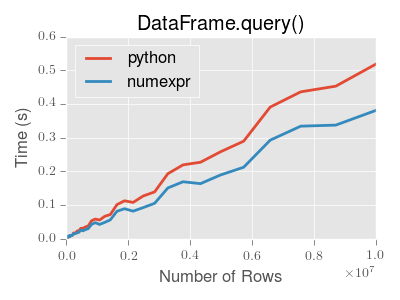
Note
You will only see the performance benefits of using the numexpr engine with DataFrame.query() if your frame has more than approximately 200,000 rows
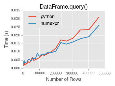
This plot was created using a DataFrame with 3 columns each containing floating point values generated using numpy.random.randn().
Take Methods
Similar to numpy ndarrays, pandas Index, Series, and DataFrame also provides the take method that retrieves elements along a given axis at the given indices. The given indices must be either a list or an ndarray of integer index positions. take will also accept negative integers as relative positions to the end of the object.
In [197]: index = Index(randint(0, 1000, 10))

In [198]: index
Out[198]: Int64Index([88, 74, 332, 407, 105, 138, 599, 893, 567, 828], dtype='int64')

In [199]: positions = [0, 9, 3]

In [200]: index[positions]
Out[200]: Int64Index([88, 828, 407], dtype='int64')

In [201]: index.take(positions)
Out[201]: Int64Index([88, 828, 407], dtype='int64')

In [202]: ser = Series(randn(10))

In [203]: ser.ix[positions]
Out[203]:
0    1.031070
9   -2.430222
3   -1.387499
dtype: float64

In [204]: ser.take(positions)
Out[204]:
0    1.031070
9   -2.430222
3   -1.387499
dtype: float64
For DataFrames, the given indices should be a 1d list or ndarray that specifies row or column positions.
In [205]: frm = DataFrame(randn(5, 3))

In [206]: frm.take([1, 4, 3])
Out[206]:
          0         1         2
1  1.263598 -2.113153  0.191012
4 -1.212239 -1.481208 -1.543384
3 -0.880774 -0.641341  2.391179

In [207]: frm.take([0, 2], axis=1)
Out[207]:
          0         2
0  1.583772 -0.710203
1  1.263598  0.191012
2  0.229587 -1.728525
3 -0.880774  2.391179
4 -1.212239 -1.543384
It is important to note that the take method on pandas objects are not intended to work on boolean indices and may return unexpected results.
In [208]: arr = randn(10)

In [209]: arr.take([False, False, True, True])
Out[209]: array([ 1.5579,  1.5579,  1.0892,  1.0892])

In [210]: arr[[0, 1]]
Out[210]: array([ 1.5579,  1.0892])

In [211]: ser = Series(randn(10))

In [212]: ser.take([False, False, True, True])
Out[212]:
0   -1.363210
0   -1.363210
1    0.623587
1    0.623587
dtype: float64

In [213]: ser.ix[[0, 1]]
Out[213]:
0   -1.363210
1    0.623587
dtype: float64
Finally, as a small note on performance, because the take method handles a narrower range of inputs, it can offer performance that is a good deal faster than fancy indexing.
Duplicate Data
If you want to identify and remove duplicate rows in a DataFrame, there are two methods that will help: duplicated and drop_duplicates. Each takes as an argument the columns to use to identify duplicated rows.
- duplicated returns a boolean vector whose length is the number of rows, and which indicates whether a row is duplicated.
- drop_duplicates removes duplicate rows.
By default, the first observed row of a duplicate set is considered unique, but each method has a take_last parameter that indicates the last observed row should be taken instead.
In [214]: df2 = DataFrame({'a' : ['one', 'one', 'two', 'three', 'two', 'one', 'six'],
   .....:                  'b' : ['x', 'y', 'y', 'x', 'y', 'x', 'x'],
   .....:                  'c' : np.random.randn(7)})
   .....:

In [215]: df2.duplicated(['a','b'])
Out[215]:
0    False
1    False
2    False
3    False
4     True
5     True
6    False
dtype: bool

In [216]: df2.drop_duplicates(['a','b'])
Out[216]:
       a  b         c
0    one  x  0.212119
1    one  y -0.398384
2    two  y -1.480017
3  three  x  0.662913
6    six  x -2.612829

In [217]: df2.drop_duplicates(['a','b'], take_last=True)
Out[217]:
       a  b         c
1    one  y -0.398384
3  three  x  0.662913
4    two  y -0.764817
5    one  x  1.568089
6    six  x -2.612829
Dictionary-like get() method
Each of Series, DataFrame, and Panel have a get method which can return a default value.
In [218]: s = Series([1,2,3], index=['a','b','c'])

In [219]: s.get('a')               # equivalent to s['a']
Out[219]: 1

In [220]: s.get('x', default=-1)
Out[220]: -1
Advanced Indexing with .ix
Note
The recent addition of .loc and .iloc have enabled users to be quite explicit about indexing choices. .ix allows a great flexibility to specify indexing locations by label and/or integer position. pandas will attempt to use any passed integer as label locations first (like what .loc would do, then to fall back on positional indexing, like what .iloc would do). See Fallback Indexing for an example.
The syntax of using .ix is identical to .loc, in Selection by Label, and .iloc in Selection by Position.
The .ix attribute takes the following inputs:
- An integer or single label, e.g. 5 or 'a'
- A list or array of labels ['a', 'b', 'c'] or integers [4, 3, 0]
- A slice object with ints 1:7 or labels 'a':'f'
- A boolean array
We’ll illustrate all of these methods. First, note that this provides a concise way of reindexing on multiple axes at once:
In [221]: subindex = dates[[3,4,5]]

In [222]: df.reindex(index=subindex, columns=['C', 'B'])
Out[222]:
                   C         B
2000-01-04 -0.042475  0.710816
2000-01-05  0.518029  1.701349
2000-01-06 -0.909180  0.227322

In [223]: df.ix[subindex, ['C', 'B']]
Out[223]:
                   C         B
2000-01-04 -0.042475  0.710816
2000-01-05  0.518029  1.701349
2000-01-06 -0.909180  0.227322
Assignment / setting values is possible when using ix:
In [224]: df2 = df.copy()

In [225]: df2.ix[subindex, ['C', 'B']] = 0

In [226]: df2
Out[226]:
                   A         B         C         D
2000-01-01  0.454389  0.854294  0.245116  0.484166
2000-01-02  0.036249 -0.546831  1.459886 -1.180301
2000-01-03  0.378125 -0.038520  1.926220  0.441177
2000-01-04  0.075871  0.000000  0.000000 -1.265025
2000-01-05 -0.677097  0.000000  0.000000 -0.592656
2000-01-06  1.482845  0.000000  0.000000  0.217613
2000-01-07  0.272681 -0.026829 -1.372775  1.109922
2000-01-08 -0.459059 -0.542800  0.869408  0.063119
Indexing with an array of integers can also be done:
In [227]: df.ix[[4,3,1]]
Out[227]:
                   A         B         C         D
2000-01-05 -0.677097  1.701349  0.518029 -0.592656
2000-01-04  0.075871  0.710816 -0.042475 -1.265025
2000-01-02  0.036249 -0.546831  1.459886 -1.180301

In [228]: df.ix[dates[[4,3,1]]]
Out[228]:
                   A         B         C         D
2000-01-05 -0.677097  1.701349  0.518029 -0.592656
2000-01-04  0.075871  0.710816 -0.042475 -1.265025
2000-01-02  0.036249 -0.546831  1.459886 -1.180301
Slicing has standard Python semantics for integer slices:
In [229]: df.ix[1:7, :2]
Out[229]:
                   A         B
2000-01-02  0.036249 -0.546831
2000-01-03  0.378125 -0.038520
2000-01-04  0.075871  0.710816
2000-01-05 -0.677097  1.701349
2000-01-06  1.482845  0.227322
2000-01-07  0.272681 -0.026829
Slicing with labels is semantically slightly different because the slice start and stop are inclusive in the label-based case:
In [230]: date1, date2 = dates[[2, 4]]

In [231]: print(date1, date2)
(Timestamp('2000-01-03 00:00:00'), Timestamp('2000-01-05 00:00:00'))

In [232]: df.ix[date1:date2]
Out[232]:
                   A         B         C         D
2000-01-03  0.378125 -0.038520  1.926220  0.441177
2000-01-04  0.075871  0.710816 -0.042475 -1.265025
2000-01-05 -0.677097  1.701349  0.518029 -0.592656

In [233]: df['A'].ix[date1:date2]
Out[233]:
2000-01-03    0.378125
2000-01-04    0.075871
2000-01-05   -0.677097
Freq: D, Name: A, dtype: float64
Getting and setting rows in a DataFrame, especially by their location, is much easier:
In [234]: df2 = df[:5].copy()

In [235]: df2.ix[3]
Out[235]:
A    0.075871
B    0.710816
C   -0.042475
D   -1.265025
Name: 2000-01-04 00:00:00, dtype: float64

In [236]: df2.ix[3] = np.arange(len(df2.columns))

In [237]: df2
Out[237]:
                   A         B         C         D
2000-01-01  0.454389  0.854294  0.245116  0.484166
2000-01-02  0.036249 -0.546831  1.459886 -1.180301
2000-01-03  0.378125 -0.038520  1.926220  0.441177
2000-01-04  0.000000  1.000000  2.000000  3.000000
2000-01-05 -0.677097  1.701349  0.518029 -0.592656
Column or row selection can be combined as you would expect with arrays of labels or even boolean vectors:
In [238]: df.ix[df['A'] > 0, 'B']
Out[238]:
2000-01-01    0.854294
2000-01-02   -0.546831
2000-01-03   -0.038520
2000-01-04    0.710816
2000-01-06    0.227322
2000-01-07   -0.026829
Name: B, dtype: float64

In [239]: df.ix[date1:date2, 'B']
Out[239]:
2000-01-03   -0.038520
2000-01-04    0.710816
2000-01-05    1.701349
Freq: D, Name: B, dtype: float64

In [240]: df.ix[date1, 'B']
Out[240]: -0.038519657937523058
Slicing with labels is closely related to the truncate method which does precisely .ix[start:stop] but returns a copy (for legacy reasons).
The select() Method
Another way to extract slices from an object is with the select method of Series, DataFrame, and Panel. This method should be used only when there is no more direct way. select takes a function which operates on labels along axis and returns a boolean. For instance:
In [241]: df.select(lambda x: x == 'A', axis=1)
Out[241]:
                   A
2000-01-01  0.454389
2000-01-02  0.036249
2000-01-03  0.378125
2000-01-04  0.075871
2000-01-05 -0.677097
2000-01-06  1.482845
2000-01-07  0.272681
2000-01-08 -0.459059
The lookup() Method
Sometimes you want to extract a set of values given a sequence of row labels and column labels, and the lookup method allows for this and returns a numpy array. For instance,
In [242]: dflookup = DataFrame(np.random.rand(20,4), columns = ['A','B','C','D'])

In [243]: dflookup.lookup(list(range(0,10,2)), ['B','C','A','B','D'])
Out[243]: array([ 0.685 ,  0.0944,  0.6808,  0.9228,  0.5607])
Float64Index
Note
As of 0.14.0, Float64Index is backed by a native float64 dtype array. Prior to 0.14.0, Float64Index was backed by an object dtype array. Using a float64 dtype in the backend speeds up arithmetic operations by about 30x and boolean indexing operations on the Float64Index itself are about 2x as fast.
New in version 0.13.0.
By default a Float64Index will be automatically created when passing floating, or mixed-integer-floating values in index creation. This enables a pure label-based slicing paradigm that makes [],ix,loc for scalar indexing and slicing work exactly the same.
In [244]: indexf = Index([1.5, 2, 3, 4.5, 5])

In [245]: indexf
Out[245]: Float64Index([1.5, 2.0, 3.0, 4.5, 5.0], dtype='float64')

In [246]: sf = Series(range(5),index=indexf)

In [247]: sf
Out[247]:
1.5    0
2.0    1
3.0    2
4.5    3
5.0    4
dtype: int32
Scalar selection for [],.ix,.loc will always be label based. An integer will match an equal float index (e.g. 3 is equivalent to 3.0)
In [248]: sf[3]
Out[248]: 2

In [249]: sf[3.0]
Out[249]: 2

In [250]: sf.ix[3]
Out[250]: 2

In [251]: sf.ix[3.0]
Out[251]: 2

In [252]: sf.loc[3]
Out[252]: 2

In [253]: sf.loc[3.0]
Out[253]: 2
The only positional indexing is via iloc
In [254]: sf.iloc[3]
Out[254]: 3
A scalar index that is not found will raise KeyError
Slicing is ALWAYS on the values of the index, for [],ix,loc and ALWAYS positional with iloc
In [255]: sf[2:4]
Out[255]:
2    1
3    2
dtype: int32

In [256]: sf.ix[2:4]
Out[256]:
2    1
3    2
dtype: int32

In [257]: sf.loc[2:4]
Out[257]:
2    1
3    2
dtype: int32

In [258]: sf.iloc[2:4]
Out[258]:
3.0    2
4.5    3
dtype: int32
In float indexes, slicing using floats is allowed
In [259]: sf[2.1:4.6]
Out[259]:
3.0    2
4.5    3
dtype: int32

In [260]: sf.loc[2.1:4.6]
Out[260]:
3.0    2
4.5    3
dtype: int32
In non-float indexes, slicing using floats will raise a TypeError
In [1]: Series(range(5))[3.5]
TypeError: the label [3.5] is not a proper indexer for this index type (Int64Index)

In [1]: Series(range(5))[3.5:4.5]
TypeError: the slice start [3.5] is not a proper indexer for this index type (Int64Index)
Using a scalar float indexer will be deprecated in a future version, but is allowed for now.
In [3]: Series(range(5))[3.0]
Out[3]: 3
Here is a typical use-case for using this type of indexing. Imagine that you have a somewhat irregular timedelta-like indexing scheme, but the data is recorded as floats. This could for example be millisecond offsets.
In [261]: dfir = concat([DataFrame(randn(5,2),
   .....:                   index=np.arange(5) * 250.0,
   .....:                   columns=list('AB')),
   .....:                DataFrame(randn(6,2),
   .....:                   index=np.arange(4,10) * 250.1,
   .....:                   columns=list('AB'))])
   .....:

In [262]: dfir
Out[262]:
               A         B
0.0    -0.781151 -2.784845
250.0  -1.201786 -0.231876
500.0  -0.142467  0.060178
750.0  -0.822858  1.876000
1000.0 -0.932658 -0.635533
1000.4  0.379122 -1.909492
1250.5 -1.431211  1.329653
1500.6 -0.562165  0.585729
1750.7 -0.544104  0.825851
2000.8 -0.062472  2.032089
2250.9  0.639479 -1.550712
Selection operations then will always work on a value basis, for all selection operators.
In [263]: dfir[0:1000.4]
Out[263]:
               A         B
0.0    -0.781151 -2.784845
250.0  -1.201786 -0.231876
500.0  -0.142467  0.060178
750.0  -0.822858  1.876000
1000.0 -0.932658 -0.635533
1000.4  0.379122 -1.909492

In [264]: dfir.loc[0:1001,'A']
Out[264]:
0.0      -0.781151
250.0    -1.201786
500.0    -0.142467
750.0    -0.822858
1000.0   -0.932658
1000.4    0.379122
Name: A, dtype: float64

In [265]: dfir.loc[1000.4]
Out[265]:
A    0.379122
B   -1.909492
Name: 1000.4, dtype: float64
You could then easily pick out the first 1 second (1000 ms) of data then.
In [266]: dfir[0:1000]
Out[266]:
             A         B
0    -0.781151 -2.784845
250  -1.201786 -0.231876
500  -0.142467  0.060178
750  -0.822858  1.876000
1000 -0.932658 -0.635533
Of course if you need integer based selection, then use iloc
In [267]: dfir.iloc[0:5]
Out[267]:
             A         B
0    -0.781151 -2.784845
250  -1.201786 -0.231876
500  -0.142467  0.060178
750  -0.822858  1.876000
1000 -0.932658 -0.635533
Returning a view versus a copy
When setting values in a pandas object, care must be taken to avoid what is called chained indexing. Here is an example.
In [268]: dfmi = DataFrame([list('abcd'),
   .....:                   list('efgh'),
   .....:                   list('ijkl'),
   .....:                   list('mnop')],
   .....:                  columns=MultiIndex.from_product([['one','two'],
   .....:                                                   ['first','second']]))
   .....:

In [269]: dfmi
Out[269]:
    one          two
  first second first second
0     a      b     c      d
1     e      f     g      h
2     i      j     k      l
3     m      n     o      p
Compare these two access methods:
In [270]: dfmi['one']['second']
Out[270]:
0    b
1    f
2    j
3    n
Name: second, dtype: object
In [271]: dfmi.loc[:,('one','second')]
Out[271]:
0    b
1    f
2    j
3    n
Name: (one, second), dtype: object
These both yield the same results, so which should you use? It is instructive to understand the order of operations on these and why method 2 (.loc) is much preferred over method 1 (chained [])
dfmi['one'] selects the first level of the columns and returns a data frame that is singly-indexed. Then another python operation dfmi_with_one['second'] selects the series indexed by 'second' happens. This is indicated by the variable dfmi_with_one because pandas sees these operations as separate events. e.g. separate calls to __getitem__, so it has to treat them as linear operations, they happen one after another.
Contrast this to df.loc[:,('one','second')] which passes a nested tuple of (slice(None),('one','second')) to a single call to __getitem__. This allows pandas to deal with this as a single entity. Furthermore this order of operations can be significantly faster, and allows one to index both axes if so desired.
Why does the assignment when using chained indexing fail!
So, why does this show the SettingWithCopy warning / and possibly not work when you do chained indexing and assignement:
dfmi['one']['second'] = value
Since the chained indexing is 2 calls, it is possible that either call may return a copy of the data because of the way it is sliced. Thus when setting, you are actually setting a copy, and not the original frame data. It is impossible for pandas to figure this out because their are 2 separate python operations that are not connected.
The SettingWithCopy warning is a ‘heuristic’ to detect this (meaning it tends to catch most cases but is simply a lightweight check). Figuring this out for real is way complicated.
The .loc operation is a single python operation, and thus can select a slice (which still may be a copy), but allows pandas to assign that slice back into the frame after it is modified, thus setting the values as you would think.
The reason for having the SettingWithCopy warning is this. Sometimes when you slice an array you will simply get a view back, which means you can set it no problem. However, even a single dtyped array can generate a copy if it is sliced in a particular way. A multi-dtyped DataFrame (meaning it has say float and object data), will almost always yield a copy. Whether a view is created is dependent on the memory layout of the array.
Evaluation order matters
Furthermore, in chained expressions, the order may determine whether a copy is returned or not. If an expression will set values on a copy of a slice, then a SettingWithCopy exception will be raised (this raise/warn behavior is new starting in 0.13.0)
You can control the action of a chained assignment via the option mode.chained_assignment, which can take the values ['raise','warn',None], where showing a warning is the default.
In [272]: dfb = DataFrame({'a' : ['one', 'one', 'two',
   .....:                         'three', 'two', 'one', 'six'],
   .....:                  'c' : np.arange(7)})
   .....:

# passed via reference (will stay)
In [273]: dfb['c'][dfb.a.str.startswith('o')] = 42
This however is operating on a copy and will not work.
>>> pd.set_option('mode.chained_assignment','warn')
>>> dfb[dfb.a.str.startswith('o')]['c'] = 42
Traceback (most recent call last)
     ...
SettingWithCopyWarning:
     A value is trying to be set on a copy of a slice from a DataFrame.
     Try using .loc[row_index,col_indexer] = value instead
A chained assignment can also crop up in setting in a mixed dtype frame.
Note
These setting rules apply to all of .loc/.iloc/.ix
This is the correct access method
In [274]: dfc = DataFrame({'A':['aaa','bbb','ccc'],'B':[1,2,3]})

In [275]: dfc.loc[0,'A'] = 11

In [276]: dfc
Out[276]:
     A  B
0   11  1
1  bbb  2
2  ccc  3
This can work at times, but is not guaranteed, and so should be avoided
In [277]: dfc = dfc.copy()

In [278]: dfc['A'][0] = 111

In [279]: dfc
Out[279]:
     A  B
0  111  1
1  bbb  2
2  ccc  3
This will not work at all, and so should be avoided
>>> pd.set_option('mode.chained_assignment','raise')
>>> dfc.loc[0]['A'] = 1111
Traceback (most recent call last)
     ...
SettingWithCopyException:
     A value is trying to be set on a copy of a slice from a DataFrame.
     Try using .loc[row_index,col_indexer] = value instead
Warning
The chained assignment warnings / exceptions are aiming to inform the user of a possibly invalid assignment. There may be false positives; situations where a chained assignment is inadvertantly reported.
Fallback indexing
Float indexes should be used only with caution. If you have a float indexed DataFrame and try to select using an integer, the row that pandas returns might not be what you expect. pandas first attempts to use the integer as a label location, but fails to find a match (because the types are not equal). pandas then falls back to back to positional indexing.
In [280]: df = pd.DataFrame(np.random.randn(4,4),
   .....:     columns=list('ABCD'), index=[1.0, 2.0, 3.0, 4.0])
   .....:

In [281]: df
Out[281]:
          A         B         C         D
1  0.903495  0.476501 -0.800435 -1.596836
2  0.242701  0.302298  1.249715 -1.524904
3 -0.726778  0.279579  1.059562 -1.783941
4 -1.377069  0.150077 -1.300946 -0.342584

In [282]: df.ix[1]
Out[282]:
A    0.903495
B    0.476501
C   -0.800435
D   -1.596836
Name: 1.0, dtype: float64
To select the row you do expect, instead use a float label or use iloc.
In [283]: df.ix[1.0]
Out[283]:
A    0.903495
B    0.476501
C   -0.800435
D   -1.596836
Name: 1.0, dtype: float64

In [284]: df.iloc[0]
Out[284]:
A    0.903495
B    0.476501
C   -0.800435
D   -1.596836
Name: 1.0, dtype: float64
Instead of using a float index, it is often better to convert to an integer index:
In [285]: df_new = df.reset_index()

In [286]: df_new[df_new['index'] == 1.0]
Out[286]:
   index         A         B         C         D
0      1  0.903495  0.476501 -0.800435 -1.596836

# now you can also do "float selection"
In [287]: df_new[(df_new['index'] >= 1.0) & (df_new['index'] < 2)]
Out[287]:
   index         A         B         C         D
0      1  0.903495  0.476501 -0.800435 -1.596836
Index objects
The pandas Index class and its subclasses can be viewed as implementing an ordered multiset. Duplicates are allowed. However, if you try to convert an Index object with duplicate entries into a set, an exception will be raised.
Index also provides the infrastructure necessary for lookups, data alignment, and reindexing. The easiest way to create an Index directly is to pass a list or other sequence to Index:
In [288]: index = Index(['e', 'd', 'a', 'b'])

In [289]: index
Out[289]: Index([u'e', u'd', u'a', u'b'], dtype='object')

In [290]: 'd' in index
Out[290]: True
You can also pass a name to be stored in the index:
In [291]: index = Index(['e', 'd', 'a', 'b'], name='something')

In [292]: index.name
Out[292]: 'something'
Starting with pandas 0.5, the name, if set, will be shown in the console display:
In [293]: index = Index(list(range(5)), name='rows')

In [294]: columns = Index(['A', 'B', 'C'], name='cols')

In [295]: df = DataFrame(np.random.randn(5, 3), index=index, columns=columns)

In [296]: df
Out[296]:
cols         A         B         C
rows
0    -1.972104  0.961460  1.222320
1     0.420597 -0.631851 -1.054843
2     0.588134  1.453543  0.668992
3    -0.024028  1.269473  1.039182
4     0.956255  1.448918  0.238470

In [297]: df['A']
Out[297]:
rows
0      -1.972104
1       0.420597
2       0.588134
3      -0.024028
4       0.956255
Name: A, dtype: float64
Set operations on Index objects
The three main operations are union (|), intersection (&), and diff (-). These can be directly called as instance methods or used via overloaded operators:
In [298]: a = Index(['c', 'b', 'a'])

In [299]: b = Index(['c', 'e', 'd'])

In [300]: a.union(b)
Out[300]: Index([u'a', u'b', u'c', u'd', u'e'], dtype='object')

In [301]: a | b
Out[301]: Index([u'a', u'b', u'c', u'd', u'e'], dtype='object')

In [302]: a & b
Out[302]: Index([u'c'], dtype='object')

In [303]: a - b
Out[303]: Index([u'a', u'b'], dtype='object')
Also available is the sym_diff (^) operation, which returns elements that appear in either idx1 or idx2 but not both. This is equivalent to the Index created by (idx1 - idx2) + (idx2 - idx1), with duplicates dropped.
In [304]: idx1 = Index([1, 2, 3, 4])

In [305]: idx2 = Index([2, 3, 4, 5])

In [306]: idx1.sym_diff(idx2)
Out[306]: Int64Index([1, 5], dtype='int64')

In [307]: idx1 ^ idx2
Out[307]: Int64Index([1, 5], dtype='int64')
Hierarchical indexing (MultiIndex)
Hierarchical indexing (also referred to as “multi-level” indexing) is brand new in the pandas 0.4 release. It is very exciting as it opens the door to some quite sophisticated data analysis and manipulation, especially for working with higher dimensional data. In essence, it enables you to store and manipulate data with an arbitrary number of dimensions in lower dimensional data structures like Series (1d) and DataFrame (2d).
In this section, we will show what exactly we mean by “hierarchical” indexing and how it integrates with the all of the pandas indexing functionality described above and in prior sections. Later, when discussing group by and pivoting and reshaping data, we’ll show non-trivial applications to illustrate how it aids in structuring data for analysis.
See the cookbook for some advanced strategies
Note
Given that hierarchical indexing is so new to the library, it is definitely “bleeding-edge” functionality but is certainly suitable for production. But, there may inevitably be some minor API changes as more use cases are explored and any weaknesses in the design / implementation are identified. pandas aims to be “eminently usable” so any feedback about new functionality like this is extremely helpful.
Creating a MultiIndex (hierarchical index) object
The MultiIndex object is the hierarchical analogue of the standard Index object which typically stores the axis labels in pandas objects. You can think of MultiIndex an array of tuples where each tuple is unique. A MultiIndex can be created from a list of arrays (using MultiIndex.from_arrays), an array of tuples (using MultiIndex.from_tuples), or a crossed set of iterables (using MultiIndex.from_product). The Index constructor will attempt to return a MultiIndex when it is passed a list of tuples. The following examples demo different ways to initialize MultiIndexes.
In [308]: arrays = [['bar', 'bar', 'baz', 'baz', 'foo', 'foo', 'qux', 'qux'],
   .....:           ['one', 'two', 'one', 'two', 'one', 'two', 'one', 'two']]
   .....:

In [309]: tuples = list(zip(*arrays))

In [310]: tuples
Out[310]:
[('bar', 'one'),
 ('bar', 'two'),
 ('baz', 'one'),
 ('baz', 'two'),
 ('foo', 'one'),
 ('foo', 'two'),
 ('qux', 'one'),
 ('qux', 'two')]

In [311]: index = MultiIndex.from_tuples(tuples, names=['first', 'second'])

In [312]: index
Out[312]:
MultiIndex(levels=[[u'bar', u'baz', u'foo', u'qux'], [u'one', u'two']],
           labels=[[0, 0, 1, 1, 2, 2, 3, 3], [0, 1, 0, 1, 0, 1, 0, 1]],
           names=[u'first', u'second'])

In [313]: s = Series(randn(8), index=index)

In [314]: s
Out[314]:
first  second
bar    one       0.174031
       two      -0.793292
baz    one       0.051545
       two       1.452842
foo    one       0.115255
       two      -0.442066
qux    one      -0.586551
       two      -0.950131
dtype: float64
When you want every pairing of the elements in two iterables, it can be easier to use the MultiIndex.from_product function:
In [315]: iterables = [['bar', 'baz', 'foo', 'qux'], ['one', 'two']]

In [316]: MultiIndex.from_product(iterables, names=['first', 'second'])
Out[316]:
MultiIndex(levels=[[u'bar', u'baz', u'foo', u'qux'], [u'one', u'two']],
           labels=[[0, 0, 1, 1, 2, 2, 3, 3], [0, 1, 0, 1, 0, 1, 0, 1]],
           names=[u'first', u'second'])
As a convenience, you can pass a list of arrays directly into Series or DataFrame to construct a MultiIndex automatically:
In [317]: arrays = [np.array(['bar', 'bar', 'baz', 'baz', 'foo', 'foo', 'qux', 'qux'])
   .....: ,
   .....:           np.array(['one', 'two', 'one', 'two', 'one', 'two', 'one', 'two'])
   .....:           ]
   .....:

In [318]: s = Series(randn(8), index=arrays)

In [319]: s
Out[319]:
bar  one    0.890610
     two   -0.170954
baz  one    0.355509
     two   -0.284458
foo  one    1.094382
     two    0.054720
qux  one    0.030047
     two    1.978266
dtype: float64

In [320]: df = DataFrame(randn(8, 4), index=arrays)

In [321]: df
Out[321]:
                0         1         2         3
bar one -0.428214 -0.116571  0.013297 -0.632840
    two -0.906030  0.064289  1.046974 -0.720532
baz one  1.100970  0.417609  0.986436 -1.277886
    two  1.534011  0.895957  1.944202 -0.547004
foo one -0.463114 -1.232976  0.881544 -1.802477
    two -0.007381 -1.219794  0.145578 -0.249321
qux one -1.046479  1.314373  0.716789  0.385795
    two -0.365315  0.370955  1.428502 -0.292967
All of the MultiIndex constructors accept a names argument which stores string names for the levels themselves. If no names are provided, None will be assigned:
In [322]: df.index.names
Out[322]: FrozenList([None, None])
This index can back any axis of a pandas object, and the number of levels of the index is up to you:
In [323]: df = DataFrame(randn(3, 8), index=['A', 'B', 'C'], columns=index)

In [324]: df
Out[324]:
first        bar                 baz                 foo                 qux  \
second       one       two       one       two       one       two       one
A      -1.250595  0.333150  0.616471 -0.915417 -0.024817 -0.795125 -0.408384
B       0.781722  0.133331 -0.298493 -1.367644  0.392245 -0.738972  0.357817
C      -0.787450  1.023850  0.475844  0.159213  1.002647  0.137063  0.287958

first
second       two
A      -1.849202
B       1.291147
C      -0.651968

In [325]: DataFrame(randn(6, 6), index=index[:6], columns=index[:6])
Out[325]:
first              bar                 baz                 foo
second             one       two       one       two       one       two
first second
bar   one    -0.422738 -0.304204  1.234844  0.692625 -2.093541  0.688230
      two     1.060943  1.152768  1.264767  0.140697  0.057916  0.405542
baz   one     0.084720  1.833111  2.103399  0.073064 -0.687485 -0.015795
      two    -0.242492  0.697262  1.151237  0.627468  0.397786 -0.811265
foo   one    -0.198387  1.403283  0.024097 -0.773295  0.463600  1.969721
      two     0.948590 -0.490665  0.313092 -0.588491  0.203166  1.632996
We’ve “sparsified” the higher levels of the indexes to make the console output a bit easier on the eyes.
It’s worth keeping in mind that there’s nothing preventing you from using tuples as atomic labels on an axis:
In [326]: Series(randn(8), index=tuples)
Out[326]:
(bar, one)   -0.557549
(bar, two)    0.126204
(baz, one)    1.643615
(baz, two)   -0.067716
(foo, one)    0.127064
(foo, two)    0.396144
(qux, one)    1.043289
(qux, two)   -0.229627
dtype: float64
The reason that the MultiIndex matters is that it can allow you to do grouping, selection, and reshaping operations as we will describe below and in subsequent areas of the documentation. As you will see in later sections, you can find yourself working with hierarchically-indexed data without creating a MultiIndex explicitly yourself. However, when loading data from a file, you may wish to generate your own MultiIndex when preparing the data set.
Note that how the index is displayed by be controlled using the multi_sparse option in pandas.set_printoptions:
In [327]: pd.set_option('display.multi_sparse', False)

In [328]: df
Out[328]:
first        bar       bar       baz       baz       foo       foo       qux  \
second       one       two       one       two       one       two       one
A      -1.250595  0.333150  0.616471 -0.915417 -0.024817 -0.795125 -0.408384
B       0.781722  0.133331 -0.298493 -1.367644  0.392245 -0.738972  0.357817
C      -0.787450  1.023850  0.475844  0.159213  1.002647  0.137063  0.287958

first        qux
second       two
A      -1.849202
B       1.291147
C      -0.651968

In [329]: pd.set_option('display.multi_sparse', True)
Reconstructing the level labels
The method get_level_values will return a vector of the labels for each location at a particular level:
In [330]: index.get_level_values(0)
Out[330]: Index([u'bar', u'bar', u'baz', u'baz', u'foo', u'foo', u'qux', u'qux'], dtype='object')

In [331]: index.get_level_values('second')
Out[331]: Index([u'one', u'two', u'one', u'two', u'one', u'two', u'one', u'two'], dtype='object')
Basic indexing on axis with MultiIndex
One of the important features of hierarchical indexing is that you can select data by a “partial” label identifying a subgroup in the data. Partial selection “drops” levels of the hierarchical index in the result in a completely analogous way to selecting a column in a regular DataFrame:
In [332]: df['bar']
Out[332]:
second       one       two
A      -1.250595  0.333150
B       0.781722  0.133331
C      -0.787450  1.023850

In [333]: df['bar', 'one']
Out[333]:
A   -1.250595
B    0.781722
C   -0.787450
Name: (bar, one), dtype: float64

In [334]: df['bar']['one']
Out[334]:
A   -1.250595
B    0.781722
C   -0.787450
Name: one, dtype: float64

In [335]: s['qux']
Out[335]:
one    0.030047
two    1.978266
dtype: float64
See Cross-section with hierarchical index for how to select on a deeper level.
Data alignment and using reindex
Operations between differently-indexed objects having MultiIndex on the axes will work as you expect; data alignment will work the same as an Index of tuples:
In [336]: s + s[:-2]
Out[336]:
bar  one    1.781221
     two   -0.341908
baz  one    0.711018
     two   -0.568917
foo  one    2.188764
     two    0.109440
qux  one         NaN
     two         NaN
dtype: float64

In [337]: s + s[::2]
Out[337]:
bar  one    1.781221
     two         NaN
baz  one    0.711018
     two         NaN
foo  one    2.188764
     two         NaN
qux  one    0.060093
     two         NaN
dtype: float64
reindex can be called with another MultiIndex or even a list or array of tuples:
In [338]: s.reindex(index[:3])
Out[338]:
first  second
bar    one       0.890610
       two      -0.170954
baz    one       0.355509
dtype: float64

In [339]: s.reindex([('foo', 'two'), ('bar', 'one'), ('qux', 'one'), ('baz', 'one')])
Out[339]:
foo  two    0.054720
bar  one    0.890610
qux  one    0.030047
baz  one    0.355509
dtype: float64
Advanced indexing with hierarchical index
Syntactically integrating MultiIndex in advanced indexing with .loc/.ix is a bit challenging, but we’ve made every effort to do so. for example the following works as you would expect:
In [340]: df = df.T

In [341]: df
Out[341]:
                     A         B         C
first second
bar   one    -1.250595  0.781722 -0.787450
      two     0.333150  0.133331  1.023850
baz   one     0.616471 -0.298493  0.475844
      two    -0.915417 -1.367644  0.159213
foo   one    -0.024817  0.392245  1.002647
      two    -0.795125 -0.738972  0.137063
qux   one    -0.408384  0.357817  0.287958
      two    -1.849202  1.291147 -0.651968

In [342]: df.loc['bar']
Out[342]:
               A         B        C
second
one    -1.250595  0.781722 -0.78745
two     0.333150  0.133331  1.02385

In [343]: df.loc['bar', 'two']
Out[343]:
A    0.333150
B    0.133331
C    1.023850
Name: (bar, two), dtype: float64
“Partial” slicing also works quite nicely.
In [344]: df.loc['baz':'foo']
Out[344]:
                     A         B         C
first second
baz   one     0.616471 -0.298493  0.475844
      two    -0.915417 -1.367644  0.159213
foo   one    -0.024817  0.392245  1.002647
      two    -0.795125 -0.738972  0.137063
You can slice with a ‘range’ of values, by providing a slice of tuples.
In [345]: df.loc[('baz', 'two'):('qux', 'one')]
Out[345]:
                     A         B         C
first second
baz   two    -0.915417 -1.367644  0.159213
foo   one    -0.024817  0.392245  1.002647
      two    -0.795125 -0.738972  0.137063
qux   one    -0.408384  0.357817  0.287958

In [346]: df.loc[('baz', 'two'):'foo']
Out[346]:
                     A         B         C
first second
baz   two    -0.915417 -1.367644  0.159213
foo   one    -0.024817  0.392245  1.002647
      two    -0.795125 -0.738972  0.137063
Passing a list of labels or tuples works similar to reindexing:
In [347]: df.ix[[('bar', 'two'), ('qux', 'one')]]
Out[347]:
                     A         B         C
first second
bar   two     0.333150  0.133331  1.023850
qux   one    -0.408384  0.357817  0.287958
Multiindexing using slicers
New in version 0.14.0.
In 0.14.0 we added a new way to slice multi-indexed objects. You can slice a multi-index by providing multiple indexers.
You can provide any of the selectors as if you are indexing by label, see Selection by Label, including slices, lists of labels, labels, and boolean indexers.
You can use slice(None) to select all the contents of that level. You do not need to specify all the deeper levels, they will be implied as slice(None).
As usual, both sides of the slicers are included as this is label indexing.
Warning
You should specify all axes in the .loc specifier, meaning the indexer for the index and for the columns. Their are some ambiguous cases where the passed indexer could be mis-interpreted as indexing both axes, rather than into say the MuliIndex for the rows.
You should do this:
df.loc[(slice('A1','A3'),.....),:]
rather than this:
df.loc[(slice('A1','A3'),.....)]
Warning
You will need to make sure that the selection axes are fully lexsorted!
In [348]: def mklbl(prefix,n):
   .....:     return ["%s%s" % (prefix,i)  for i in range(n)]
   .....:

In [349]: miindex = MultiIndex.from_product([mklbl('A',4),
   .....:                                    mklbl('B',2),
   .....:                                    mklbl('C',4),
   .....:                                    mklbl('D',2)])
   .....:

In [350]: micolumns = MultiIndex.from_tuples([('a','foo'),('a','bar'),
   .....:                                     ('b','foo'),('b','bah')],
   .....:                                      names=['lvl0', 'lvl1'])
   .....:

In [351]: dfmi = DataFrame(np.arange(len(miindex)*len(micolumns)).reshape((len(miindex),len(micolumns))),
   .....:                  index=miindex,
   .....:                  columns=micolumns).sortlevel().sortlevel(axis=1)
   .....:

In [352]: dfmi
Out[352]:
lvl0           a         b
lvl1         bar  foo  bah  foo
A0 B0 C0 D0    1    0    3    2
         D1    5    4    7    6
      C1 D0    9    8   11   10
         D1   13   12   15   14
      C2 D0   17   16   19   18
         D1   21   20   23   22
      C3 D0   25   24   27   26
...          ...  ...  ...  ...
A3 B1 C0 D1  229  228  231  230
      C1 D0  233  232  235  234
         D1  237  236  239  238
      C2 D0  241  240  243  242
         D1  245  244  247  246
      C3 D0  249  248  251  250
         D1  253  252  255  254

[64 rows x 4 columns]
Basic multi-index slicing using slices, lists, and labels.
In [353]: dfmi.loc[(slice('A1','A3'),slice(None), ['C1','C3']),:]
Out[353]:
lvl0           a         b
lvl1         bar  foo  bah  foo
A1 B0 C1 D0   73   72   75   74
         D1   77   76   79   78
      C3 D0   89   88   91   90
         D1   93   92   95   94
   B1 C1 D0  105  104  107  106
         D1  109  108  111  110
      C3 D0  121  120  123  122
...          ...  ...  ...  ...
A3 B0 C1 D1  205  204  207  206
      C3 D0  217  216  219  218
         D1  221  220  223  222
   B1 C1 D0  233  232  235  234
         D1  237  236  239  238
      C3 D0  249  248  251  250
         D1  253  252  255  254

[24 rows x 4 columns]
You can use a pd.IndexSlice to shortcut the creation of these slices
In [354]: idx = pd.IndexSlice

In [355]: dfmi.loc[idx[:,:,['C1','C3']],idx[:,'foo']]
Out[355]:
lvl0           a    b
lvl1         foo  foo
A0 B0 C1 D0    8   10
         D1   12   14
      C3 D0   24   26
         D1   28   30
   B1 C1 D0   40   42
         D1   44   46
      C3 D0   56   58
...          ...  ...
A3 B0 C1 D1  204  206
      C3 D0  216  218
         D1  220  222
   B1 C1 D0  232  234
         D1  236  238
      C3 D0  248  250
         D1  252  254

[32 rows x 2 columns]
It is possible to perform quite complicated selections using this method on multiple axes at the same time.
In [356]: dfmi.loc['A1',(slice(None),'foo')]
Out[356]:
lvl0        a    b
lvl1      foo  foo
B0 C0 D0   64   66
      D1   68   70
   C1 D0   72   74
      D1   76   78
   C2 D0   80   82
      D1   84   86
   C3 D0   88   90
...       ...  ...
B1 C0 D1  100  102
   C1 D0  104  106
      D1  108  110
   C2 D0  112  114
      D1  116  118
   C3 D0  120  122
      D1  124  126

[16 rows x 2 columns]

In [357]: dfmi.loc[idx[:,:,['C1','C3']],idx[:,'foo']]
Out[357]:
lvl0           a    b
lvl1         foo  foo
A0 B0 C1 D0    8   10
         D1   12   14
      C3 D0   24   26
         D1   28   30
   B1 C1 D0   40   42
         D1   44   46
      C3 D0   56   58
...          ...  ...
A3 B0 C1 D1  204  206
      C3 D0  216  218
         D1  220  222
   B1 C1 D0  232  234
         D1  236  238
      C3 D0  248  250
         D1  252  254

[32 rows x 2 columns]
Using a boolean indexer you can provide selection related to the values.
In [358]: mask = dfmi[('a','foo')]>200

In [359]: dfmi.loc[idx[mask,:,['C1','C3']],idx[:,'foo']]
Out[359]:
lvl0           a    b
lvl1         foo  foo
A3 B0 C1 D1  204  206
      C3 D0  216  218
         D1  220  222
   B1 C1 D0  232  234
         D1  236  238
      C3 D0  248  250
         D1  252  254
You can also specify the axis argument to .loc to interpret the passed slicers on a single axis.
In [360]: dfmi.loc(axis=0)[:,:,['C1','C3']]
Out[360]:
lvl0           a         b
lvl1         bar  foo  bah  foo
A0 B0 C1 D0    9    8   11   10
         D1   13   12   15   14
      C3 D0   25   24   27   26
         D1   29   28   31   30
   B1 C1 D0   41   40   43   42
         D1   45   44   47   46
      C3 D0   57   56   59   58
...          ...  ...  ...  ...
A3 B0 C1 D1  205  204  207  206
      C3 D0  217  216  219  218
         D1  221  220  223  222
   B1 C1 D0  233  232  235  234
         D1  237  236  239  238
      C3 D0  249  248  251  250
         D1  253  252  255  254

[32 rows x 4 columns]
Furthermore you can set the values using these methods
In [361]: df2 = dfmi.copy()

In [362]: df2.loc(axis=0)[:,:,['C1','C3']] = -10

In [363]: df2
Out[363]:
lvl0           a         b
lvl1         bar  foo  bah  foo
A0 B0 C0 D0    1    0    3    2
         D1    5    4    7    6
      C1 D0  -10  -10  -10  -10
         D1  -10  -10  -10  -10
      C2 D0   17   16   19   18
         D1   21   20   23   22
      C3 D0  -10  -10  -10  -10
...          ...  ...  ...  ...
A3 B1 C0 D1  229  228  231  230
      C1 D0  -10  -10  -10  -10
         D1  -10  -10  -10  -10
      C2 D0  241  240  243  242
         D1  245  244  247  246
      C3 D0  -10  -10  -10  -10
         D1  -10  -10  -10  -10

[64 rows x 4 columns]
You can use a right-hand-side of an alignable object as well.
In [364]: df2 = dfmi.copy()

In [365]: df2.loc[idx[:,:,['C1','C3']],:] = df2*1000

In [366]: df2
Out[366]:
lvl0              a               b
lvl1            bar     foo     bah     foo
A0 B0 C0 D0       1       0       3       2
         D1       5       4       7       6
      C1 D0    1000       0    3000    2000
         D1    5000    4000    7000    6000
      C2 D0      17      16      19      18
         D1      21      20      23      22
      C3 D0    9000    8000   11000   10000
...             ...     ...     ...     ...
A3 B1 C0 D1     229     228     231     230
      C1 D0  113000  112000  115000  114000
         D1  117000  116000  119000  118000
      C2 D0     241     240     243     242
         D1     245     244     247     246
      C3 D0  121000  120000  123000  122000
         D1  125000  124000  127000  126000

[64 rows x 4 columns]
Cross-section with hierarchical index
The xs method of DataFrame additionally takes a level argument to make selecting data at a particular level of a MultiIndex easier.
In [367]: df.xs('one', level='second')
Out[367]:
              A         B         C
first
bar   -1.250595  0.781722 -0.787450
baz    0.616471 -0.298493  0.475844
foo   -0.024817  0.392245  1.002647
qux   -0.408384  0.357817  0.287958
# using the slicers (new in 0.14.0)
In [368]: df.loc[(slice(None),'one'),:]
Out[368]:
                     A         B         C
first second
bar   one    -1.250595  0.781722 -0.787450
baz   one     0.616471 -0.298493  0.475844
foo   one    -0.024817  0.392245  1.002647
qux   one    -0.408384  0.357817  0.287958
You can also select on the columns with xs(), by providing the axis argument
In [369]: df = df.T

In [370]: df.xs('one', level='second', axis=1)
Out[370]:
first       bar       baz       foo       qux
A     -1.250595  0.616471 -0.024817 -0.408384
B      0.781722 -0.298493  0.392245  0.357817
C     -0.787450  0.475844  1.002647  0.287958
# using the slicers (new in 0.14.0)
In [371]: df.loc[:,(slice(None),'one')]
Out[371]:
first        bar       baz       foo       qux
second       one       one       one       one
A      -1.250595  0.616471 -0.024817 -0.408384
B       0.781722 -0.298493  0.392245  0.357817
C      -0.787450  0.475844  1.002647  0.287958
xs() also allows selection with multiple keys
In [372]: df.xs(('one', 'bar'), level=('second', 'first'), axis=1)
Out[372]:
first        bar
second       one
A      -1.250595
B       0.781722
C      -0.787450
# using the slicers (new in 0.14.0)
In [373]: df.loc[:,('bar','one')]
Out[373]:
A   -1.250595
B    0.781722
C   -0.787450
Name: (bar, one), dtype: float64
New in version 0.13.0.
You can pass drop_level=False to xs() to retain the level that was selected
In [374]: df.xs('one', level='second', axis=1, drop_level=False)
Out[374]:
first        bar       baz       foo       qux
second       one       one       one       one
A      -1.250595  0.616471 -0.024817 -0.408384
B       0.781722 -0.298493  0.392245  0.357817
C      -0.787450  0.475844  1.002647  0.287958
versus the result with drop_level=True (the default value)
In [375]: df.xs('one', level='second', axis=1, drop_level=True)
Out[375]:
first       bar       baz       foo       qux
A     -1.250595  0.616471 -0.024817 -0.408384
B      0.781722 -0.298493  0.392245  0.357817
C     -0.787450  0.475844  1.002647  0.287958
Advanced reindexing and alignment with hierarchical index
The parameter level has been added to the reindex and align methods of pandas objects. This is useful to broadcast values across a level. For instance:
In [376]: midx = MultiIndex(levels=[['zero', 'one'], ['x','y']],
   .....:                   labels=[[1,1,0,0],[1,0,1,0]])
   .....:

In [377]: df = DataFrame(randn(4,2), index=midx)

In [378]: print(df)
               0         1
one  y  0.158186 -0.281965
     x  1.255148  3.063464
zero y  0.304771 -0.766820
     x -0.878886  0.105620

In [379]: df2 = df.mean(level=0)

In [380]: print(df2)
             0         1
zero -0.287058 -0.330600
one   0.706667  1.390749

In [381]: print(df2.reindex(df.index, level=0))
               0         1
one  y  0.706667  1.390749
     x  0.706667  1.390749
zero y -0.287058 -0.330600
     x -0.287058 -0.330600

In [382]: df_aligned, df2_aligned = df.align(df2, level=0)

In [383]: print(df_aligned)
               0         1
one  y  0.158186 -0.281965
     x  1.255148  3.063464
zero y  0.304771 -0.766820
     x -0.878886  0.105620

In [384]: print(df2_aligned)
               0         1
one  y  0.706667  1.390749
     x  0.706667  1.390749
zero y -0.287058 -0.330600
     x -0.287058 -0.330600
The need for sortedness with MultiIndex
Caveat emptor: the present implementation of MultiIndex requires that the labels be sorted for some of the slicing / indexing routines to work correctly. You can think about breaking the axis into unique groups, where at the hierarchical level of interest, each distinct group shares a label, but no two have the same label. However, the MultiIndex does not enforce this: you are responsible for ensuring that things are properly sorted. There is an important new method sortlevel to sort an axis within a MultiIndex so that its labels are grouped and sorted by the original ordering of the associated factor at that level. Note that this does not necessarily mean the labels will be sorted lexicographically!
In [385]: import random; random.shuffle(tuples)

In [386]: s = Series(randn(8), index=MultiIndex.from_tuples(tuples))

In [387]: s
Out[387]:
baz  two    0.248051
     one    1.691324
bar  two   -0.151669
foo  two    1.766577
qux  two    0.604424
bar  one   -0.337383
foo  one    0.072225
qux  one   -1.348017
dtype: float64

In [388]: s.sortlevel(0)
Out[388]:
bar  one   -0.337383
     two   -0.151669
baz  one    1.691324
     two    0.248051
foo  one    0.072225
     two    1.766577
qux  one   -1.348017
     two    0.604424
dtype: float64

In [389]: s.sortlevel(1)
Out[389]:
bar  one   -0.337383
baz  one    1.691324
foo  one    0.072225
qux  one   -1.348017
bar  two   -0.151669
baz  two    0.248051
foo  two    1.766577
qux  two    0.604424
dtype: float64
Note, you may also pass a level name to sortlevel if the MultiIndex levels are named.
In [390]: s.index.set_names(['L1', 'L2'], inplace=True)

In [391]: s.sortlevel(level='L1')
Out[391]:
L1   L2
bar  one   -0.337383
     two   -0.151669
baz  one    1.691324
     two    0.248051
foo  one    0.072225
     two    1.766577
qux  one   -1.348017
     two    0.604424
dtype: float64

In [392]: s.sortlevel(level='L2')
Out[392]:
L1   L2
bar  one   -0.337383
baz  one    1.691324
foo  one    0.072225
qux  one   -1.348017
bar  two   -0.151669
baz  two    0.248051
foo  two    1.766577
qux  two    0.604424
dtype: float64
Some indexing will work even if the data are not sorted, but will be rather inefficient and will also return a copy of the data rather than a view:
In [393]: s['qux']
Out[393]:
L2
two    0.604424
one   -1.348017
dtype: float64

In [394]: s.sortlevel(1)['qux']
Out[394]:
L2
one   -1.348017
two    0.604424
dtype: float64
On higher dimensional objects, you can sort any of the other axes by level if they have a MultiIndex:
In [395]: df.T.sortlevel(1, axis=1)
Out[395]:
       zero       one      zero       one
          x         x         y         y
0 -0.878886  1.255148  0.304771  0.158186
1  0.105620  3.063464 -0.766820 -0.281965
The MultiIndex object has code to explicity check the sort depth. Thus, if you try to index at a depth at which the index is not sorted, it will raise an exception. Here is a concrete example to illustrate this:
In [396]: tuples = [('a', 'a'), ('a', 'b'), ('b', 'a'), ('b', 'b')]

In [397]: idx = MultiIndex.from_tuples(tuples)

In [398]: idx.lexsort_depth
Out[398]: 2

In [399]: reordered = idx[[1, 0, 3, 2]]

In [400]: reordered.lexsort_depth
Out[400]: 1

In [401]: s = Series(randn(4), index=reordered)

In [402]: s.ix['a':'a']
Out[402]:
a  b   -0.157935
   a    0.766538
dtype: float64
However:
>>> s.ix[('a', 'b'):('b', 'a')]
Traceback (most recent call last)
     ...
KeyError: Key length (3) was greater than MultiIndex lexsort depth (2)
Swapping levels with swaplevel()
The swaplevel function can switch the order of two levels:
In [403]: df[:5]
Out[403]:
               0         1
one  y  0.158186 -0.281965
     x  1.255148  3.063464
zero y  0.304771 -0.766820
     x -0.878886  0.105620

In [404]: df[:5].swaplevel(0, 1, axis=0)
Out[404]:
               0         1
y one   0.158186 -0.281965
x one   1.255148  3.063464
y zero  0.304771 -0.766820
x zero -0.878886  0.105620
Reordering levels with reorder_levels()
The reorder_levels function generalizes the swaplevel function, allowing you to permute the hierarchical index levels in one step:
In [405]: df[:5].reorder_levels([1,0], axis=0)
Out[405]:
               0         1
y one   0.158186 -0.281965
x one   1.255148  3.063464
y zero  0.304771 -0.766820
x zero -0.878886  0.105620
Some gory internal details
Internally, the MultiIndex consists of a few things: the levels, the integer labels, and the level names:
In [406]: index
Out[406]:
MultiIndex(levels=[[u'bar', u'baz', u'foo', u'qux'], [u'one', u'two']],
           labels=[[0, 0, 1, 1, 2, 2, 3, 3], [0, 1, 0, 1, 0, 1, 0, 1]],
           names=[u'first', u'second'])

In [407]: index.levels
Out[407]: FrozenList([[u'bar', u'baz', u'foo', u'qux'], [u'one', u'two']])

In [408]: index.labels
Out[408]: FrozenList([[0, 0, 1, 1, 2, 2, 3, 3], [0, 1, 0, 1, 0, 1, 0, 1]])

In [409]: index.names
Out[409]: FrozenList([u'first', u'second'])
You can probably guess that the labels determine which unique element is identified with that location at each layer of the index. It’s important to note that sortedness is determined solely from the integer labels and does not check (or care) whether the levels themselves are sorted. Fortunately, the constructors from_tuples and from_arrays ensure that this is true, but if you compute the levels and labels yourself, please be careful.
Setting index metadata (name(s), levels, labels)
New in version 0.13.0.
Indexes are “mostly immutable”, but it is possible to set and change their metadata, like the index name (or, for MultiIndex, levels and labels).
You can use the rename, set_names, set_levels, and set_labels to set these attributes directly. They default to returning a copy; however, you can specify inplace=True to have the data change inplace.
In [410]: ind = Index([1, 2, 3])

In [411]: ind.rename("apple")
Out[411]: Int64Index([1, 2, 3], dtype='int64')

In [412]: ind
Out[412]: Int64Index([1, 2, 3], dtype='int64')

In [413]: ind.set_names(["apple"], inplace=True)

In [414]: ind.name = "bob"

In [415]: ind
Out[415]: Int64Index([1, 2, 3], dtype='int64')
Adding an index to an existing DataFrame
Occasionally you will load or create a data set into a DataFrame and want to add an index after you’ve already done so. There are a couple of different ways.
Add an index using DataFrame columns
DataFrame has a set_index method which takes a column name (for a regular Index) or a list of column names (for a MultiIndex), to create a new, indexed DataFrame:
In [416]: data
Out[416]:
     a    b  c  d
0  bar  one  z  1
1  bar  two  y  2
2  foo  one  x  3
3  foo  two  w  4

In [417]: indexed1 = data.set_index('c')

In [418]: indexed1
Out[418]:
     a    b  d
c
z  bar  one  1
y  bar  two  2
x  foo  one  3
w  foo  two  4

In [419]: indexed2 = data.set_index(['a', 'b'])

In [420]: indexed2
Out[420]:
         c  d
a   b
bar one  z  1
    two  y  2
foo one  x  3
    two  w  4
The append keyword option allow you to keep the existing index and append the given columns to a MultiIndex:
In [421]: frame = data.set_index('c', drop=False)

In [422]: frame = frame.set_index(['a', 'b'], append=True)

In [423]: frame
Out[423]:
           c  d
c a   b
z bar one  z  1
y bar two  y  2
x foo one  x  3
w foo two  w  4
Other options in set_index allow you not drop the index columns or to add the index in-place (without creating a new object):
In [424]: data.set_index('c', drop=False)
Out[424]:
     a    b  c  d
c
z  bar  one  z  1
y  bar  two  y  2
x  foo  one  x  3
w  foo  two  w  4

In [425]: data.set_index(['a', 'b'], inplace=True)

In [426]: data
Out[426]:
         c  d
a   b
bar one  z  1
    two  y  2
foo one  x  3
    two  w  4
Remove / reset the index, reset_index
As a convenience, there is a new function on DataFrame called reset_index which transfers the index values into the DataFrame’s columns and sets a simple integer index. This is the inverse operation to set_index
In [427]: data
Out[427]:
         c  d
a   b
bar one  z  1
    two  y  2
foo one  x  3
    two  w  4

In [428]: data.reset_index()
Out[428]:
     a    b  c  d
0  bar  one  z  1
1  bar  two  y  2
2  foo  one  x  3
3  foo  two  w  4
The output is more similar to a SQL table or a record array. The names for the columns derived from the index are the ones stored in the names attribute.
You can use the level keyword to remove only a portion of the index:
In [429]: frame
Out[429]:
           c  d
c a   b
z bar one  z  1
y bar two  y  2
x foo one  x  3
w foo two  w  4

In [430]: frame.reset_index(level=1)
Out[430]:
         a  c  d
c b
z one  bar  z  1
y two  bar  y  2
x one  foo  x  3
w two  foo  w  4
reset_index takes an optional parameter drop which if true simply discards the index, instead of putting index values in the DataFrame’s columns.
Note
The reset_index method used to be called delevel which is now deprecated.
Adding an ad hoc index
If you create an index yourself, you can just assign it to the index field:
data.index = index
Indexing internal details
Note
The following is largely relevant for those actually working on the pandas codebase. The source code is still the best place to look at the specifics of how things are implemented.
In pandas there are a few objects implemented which can serve as valid containers for the axis labels:
- Index: the generic “ordered set” object, an ndarray of object dtype assuming nothing about its contents. The labels must be hashable (and likely immutable) and unique. Populates a dict of label to location in Cython to do
lookups.
- Int64Index: a version of Index highly optimized for 64-bit integer data, such as time stamps
- MultiIndex: the standard hierarchical index object
- PeriodIndex: An Index object with Period elements
- DatetimeIndex: An Index object with Timestamp elements
- date_range: fixed frequency date range generated from a time rule or DateOffset. An ndarray of Python datetime objects
The motivation for having an Index class in the first place was to enable different implementations of indexing. This means that it’s possible for you, the user, to implement a custom Index subclass that may be better suited to a particular application than the ones provided in pandas.
From an internal implementation point of view, the relevant methods that an Index must define are one or more of the following (depending on how incompatible the new object internals are with the Index functions):
- get_loc: returns an “indexer” (an integer, or in some cases a slice object) for a label
- slice_locs: returns the “range” to slice between two labels
- get_indexer: Computes the indexing vector for reindexing / data alignment purposes. See the source / docstrings for more on this
- get_indexer_non_unique: Computes the indexing vector for reindexing / data alignment purposes when the index is non-unique. See the source / docstrings for more on this
- reindex: Does any pre-conversion of the input index then calls get_indexer
- union, intersection: computes the union or intersection of two Index objects
- insert: Inserts a new label into an Index, yielding a new object
- delete: Delete a label, yielding a new object
- drop: Deletes a set of labels
- take: Analogous to ndarray.take