Intro to Data Structures
We’ll start with a quick, non-comprehensive overview of the fundamental data structures in pandas to get you started. The fundamental behavior about data types, indexing, and axis labeling / alignment apply across all of the objects. To get started, import numpy and load pandas into your namespace:
In [1]: import numpy as np

In [2]: import pandas as pd
Here is a basic tenet to keep in mind: data alignment is intrinsic. The link between labels and data will not be broken unless done so explicitly by you.
We’ll give a brief intro to the data structures, then consider all of the broad categories of functionality and methods in separate sections.
Series
Series is a one-dimensional labeled array capable of holding any data
type (integers, strings, floating point numbers, Python objects, etc.). The axis
labels are collectively referred to as the index. The basic method to create a Series is to call:
>>> s = pd.Series(data, index=index)
Here, data can be many different things:
- a Python dict
- an ndarray
- a scalar value (like 5)
The passed index is a list of axis labels. Thus, this separates into a few cases depending on what data is:
From ndarray
If data is an ndarray, index must be the same length as data. If no
index is passed, one will be created having values [0, ..., len(data) - 1].
In [3]: s = pd.Series(np.random.randn(5), index=['a', 'b', 'c', 'd', 'e'])
In [4]: s
Out[4]:
a 0.2941
b 0.2869
c 1.7098
d -0.2126
e 0.2696
dtype: float64
In [5]: s.index
������������������������������������������������������������������������������������Out[5]: Index(['a', 'b', 'c', 'd', 'e'], dtype='object')
In [6]: pd.Series(np.random.randn(5))
���������������������������������������������������������������������������������������������������������������������������������������������Out[6]:
0 -0.4531
1 -1.8215
2 -0.1263
3 -0.1533
4 0.4055
dtype: float64
Note
Starting in v0.8.0, pandas supports non-unique index values. If an operation that does not support duplicate index values is attempted, an exception will be raised at that time. The reason for being lazy is nearly all performance-based (there are many instances in computations, like parts of GroupBy, where the index is not used).
From dict
If data is a dict, if index is passed the values in data corresponding
to the labels in the index will be pulled out. Otherwise, an index will be
constructed from the sorted keys of the dict, if possible.
In [7]: d = {'a' : 0., 'b' : 1., 'c' : 2.}
In [8]: pd.Series(d)
Out[8]:
a 0.0
b 1.0
c 2.0
dtype: float64
In [9]: pd.Series(d, index=['b', 'c', 'd', 'a'])
���������������������������������������������������Out[9]:
b 1.0
c 2.0
d NaN
a 0.0
dtype: float64
Note
NaN (not a number) is the standard missing data marker used in pandas
From scalar value If data is a scalar value, an index must be
provided. The value will be repeated to match the length of index
In [10]: pd.Series(5., index=['a', 'b', 'c', 'd', 'e'])
Out[10]:
a    5.0
b    5.0
c    5.0
d    5.0
e    5.0
dtype: float64
Series is ndarray-like
Series acts very similarly to a ndarray, and is a valid argument to most NumPy functions.
However, things like slicing also slice the index.
In [11]: s[0]
Out[11]: 0.29413876297575337
In [12]: s[:3]
�����������������������������Out[12]:
a 0.2941
b 0.2869
c 1.7098
dtype: float64
In [13]: s[s > s.median()]
������������������������������������������������������������������������������������������Out[13]:
a 0.2941
c 1.7098
dtype: float64
In [14]: s[[4, 3, 1]]
�������������������������������������������������������������������������������������������������������������������������������������������Out[14]:
e 0.2696
d -0.2126
b 0.2869
dtype: float64
In [15]: np.exp(s)
��������������������������������������������������������������������������������������������������������������������������������������������������������������������������������������������������������Out[15]:
a 1.3420
b 1.3323
c 5.5276
d 0.8085
e 1.3094
dtype: float64
We will address array-based indexing in a separate section.
Series is dict-like
A Series is like a fixed-size dict in that you can get and set values by index label:
In [16]: s['a']
Out[16]: 0.29413876297575337
In [17]: s['e'] = 12.
In [18]: s
Out[18]:
a 0.2941
b 0.2869
c 1.7098
d -0.2126
e 12.0000
dtype: float64
In [19]: 'e' in s
������������������������������������������������������������������������������������������Out[19]: True
In [20]: 'f' in s
��������������������������������������������������������������������������������������������������������Out[20]: False
If a label is not contained, an exception is raised:
>>> s['f']
KeyError: 'f'
Using the get method, a missing label will return None or specified default:
In [21]: s.get('f')

In [22]: s.get('f', np.nan)
Out[22]: nan
See also the section on attribute access.
Vectorized operations and label alignment with Series
When doing data analysis, as with raw NumPy arrays looping through Series value-by-value is usually not necessary. Series can also be passed into most NumPy methods expecting an ndarray.
In [23]: s + s
Out[23]:
a 0.5883
b 0.5739
c 3.4195
d -0.4252
e 24.0000
dtype: float64
In [24]: s * 2
������������������������������������������������������������������������������������������Out[24]:
a 0.5883
b 0.5739
c 3.4195
d -0.4252
e 24.0000
dtype: float64
In [25]: np.exp(s)
������������������������������������������������������������������������������������������������������������������������������������������������������������������������������������Out[25]:
a 1.3420
b 1.3323
c 5.5276
d 0.8085
e 162754.7914
dtype: float64
A key difference between Series and ndarray is that operations between Series automatically align the data based on label. Thus, you can write computations without giving consideration to whether the Series involved have the same labels.
In [26]: s[1:] + s[:-1]
Out[26]:
a       NaN
b    0.5739
c    3.4195
d   -0.4252
e       NaN
dtype: float64
The result of an operation between unaligned Series will have the union of
the indexes involved. If a label is not found in one Series or the other, the
result will be marked as missing NaN. Being able to write code without doing
any explicit data alignment grants immense freedom and flexibility in
interactive data analysis and research. The integrated data alignment features
of the pandas data structures set pandas apart from the majority of related
tools for working with labeled data.
Note
In general, we chose to make the default result of operations between differently indexed objects yield the union of the indexes in order to avoid loss of information. Having an index label, though the data is missing, is typically important information as part of a computation. You of course have the option of dropping labels with missing data via the dropna function.
Name attribute
Series can also have a name attribute:
In [27]: s = pd.Series(np.random.randn(5), name='something')
In [28]: s
Out[28]:
0 -0.5046
1 1.4051
2 0.7781
3 -0.7990
4 -0.6707
Name: something, dtype: float64
In [29]: s.name
������������������������������������������������������������������������������������������������������Out[29]: 'something'
The Series name will be assigned automatically in many cases, in particular
when taking 1D slices of DataFrame as you will see below.
New in version 0.18.0.
You can rename a Series with the pandas.Series.rename() method.
In [30]: s2 = s.rename("different")

In [31]: s2.name
Out[31]: 'different'
Note that s and s2 refer to different objects.
DataFrame
DataFrame is a 2-dimensional labeled data structure with columns of potentially different types. You can think of it like a spreadsheet or SQL table, or a dict of Series objects. It is generally the most commonly used pandas object. Like Series, DataFrame accepts many different kinds of input:
- Dict of 1D ndarrays, lists, dicts, or Series
- 2-D numpy.ndarray
- Structured or record ndarray
- A
Series- Another
DataFrame
Along with the data, you can optionally pass index (row labels) and columns (column labels) arguments. If you pass an index and / or columns, you are guaranteeing the index and / or columns of the resulting DataFrame. Thus, a dict of Series plus a specific index will discard all data not matching up to the passed index.
If axis labels are not passed, they will be constructed from the input data based on common sense rules.
From dict of Series or dicts
The result index will be the union of the indexes of the various Series. If there are any nested dicts, these will be first converted to Series. If no columns are passed, the columns will be the sorted list of dict keys.
In [32]: d = {'one' : pd.Series([1., 2., 3.], index=['a', 'b', 'c']),
....: 'two' : pd.Series([1., 2., 3., 4.], index=['a', 'b', 'c', 'd'])}
....:
In [33]: df = pd.DataFrame(d)
In [34]: df
Out[34]:
one two
a 1.0 1.0
b 2.0 2.0
c 3.0 3.0
d NaN 4.0
In [35]: pd.DataFrame(d, index=['d', 'b', 'a'])
����������������������������������������������������������������������Out[35]:
one two
d NaN 4.0
b 2.0 2.0
a 1.0 1.0
In [36]: pd.DataFrame(d, index=['d', 'b', 'a'], columns=['two', 'three'])
��������������������������������������������������������������������������������������������������������������������������������Out[36]:
two three
d 4.0 NaN
b 2.0 NaN
a 1.0 NaN
The row and column labels can be accessed respectively by accessing the index and columns attributes:
Note
When a particular set of columns is passed along with a dict of data, the passed columns override the keys in the dict.
In [37]: df.index
Out[37]: Index(['a', 'b', 'c', 'd'], dtype='object')
In [38]: df.columns
�����������������������������������������������������Out[38]: Index(['one', 'two'], dtype='object')
From dict of ndarrays / lists
The ndarrays must all be the same length. If an index is passed, it must
clearly also be the same length as the arrays. If no index is passed, the
result will be range(n), where n is the array length.
In [39]: d = {'one' : [1., 2., 3., 4.],
....: 'two' : [4., 3., 2., 1.]}
....:
In [40]: pd.DataFrame(d)
Out[40]:
one two
0 1.0 4.0
1 2.0 3.0
2 3.0 2.0
3 4.0 1.0
In [41]: pd.DataFrame(d, index=['a', 'b', 'c', 'd'])
����������������������������������������������������������������������Out[41]:
one two
a 1.0 4.0
b 2.0 3.0
c 3.0 2.0
d 4.0 1.0
From structured or record array
This case is handled identically to a dict of arrays.
In [42]: data = np.zeros((2,), dtype=[('A', 'i4'),('B', 'f4'),('C', 'a10')])
In [43]: data[:] = [(1,2.,'Hello'), (2,3.,"World")]
In [44]: pd.DataFrame(data)
Out[44]:
A B C
0 1 2.0 b'Hello'
1 2 3.0 b'World'
In [45]: pd.DataFrame(data, index=['first', 'second'])
����������������������������������������������������������������������Out[45]:
A B C
first 1 2.0 b'Hello'
second 2 3.0 b'World'
In [46]: pd.DataFrame(data, columns=['C', 'A', 'B'])
�����������������������������������������������������������������������������������������������������������������������������������������������������������Out[46]:
C A B
0 b'Hello' 1 2.0
1 b'World' 2 3.0
Note
DataFrame is not intended to work exactly like a 2-dimensional NumPy ndarray.
From a list of dicts
In [47]: data2 = [{'a': 1, 'b': 2}, {'a': 5, 'b': 10, 'c': 20}]
In [48]: pd.DataFrame(data2)
Out[48]:
a b c
0 1 2 NaN
1 5 10 20.0
In [49]: pd.DataFrame(data2, index=['first', 'second'])
�������������������������������������������������������Out[49]:
a b c
first 1 2 NaN
second 5 10 20.0
In [50]: pd.DataFrame(data2, columns=['a', 'b'])
�����������������������������������������������������������������������������������������������������������������������������Out[50]:
a b
0 1 2
1 5 10
From a dict of tuples
You can automatically create a multi-indexed frame by passing a tuples dictionary
In [51]: pd.DataFrame({('a', 'b'): {('A', 'B'): 1, ('A', 'C'): 2},
   ....:               ('a', 'a'): {('A', 'C'): 3, ('A', 'B'): 4},
   ....:               ('a', 'c'): {('A', 'B'): 5, ('A', 'C'): 6},
   ....:               ('b', 'a'): {('A', 'C'): 7, ('A', 'B'): 8},
   ....:               ('b', 'b'): {('A', 'D'): 9, ('A', 'B'): 10}})
   ....:
Out[51]:
       a              b
       a    b    c    a     b
A B  4.0  1.0  5.0  8.0  10.0
  C  3.0  2.0  6.0  7.0   NaN
  D  NaN  NaN  NaN  NaN   9.0
From a Series
The result will be a DataFrame with the same index as the input Series, and with one column whose name is the original name of the Series (only if no other column name provided).
Missing Data
Much more will be said on this topic in the Missing data
section. To construct a DataFrame with missing data, use np.nan for those
values which are missing. Alternatively, you may pass a numpy.MaskedArray
as the data argument to the DataFrame constructor, and its masked entries will
be considered missing.
Alternate Constructors
DataFrame.from_dict
DataFrame.from_dict takes a dict of dicts or a dict of array-like sequences
and returns a DataFrame. It operates like the DataFrame constructor except
for the orient parameter which is 'columns' by default, but which can be
set to 'index' in order to use the dict keys as row labels.
DataFrame.from_records
DataFrame.from_records takes a list of tuples or an ndarray with structured
dtype. Works analogously to the normal DataFrame constructor, except that
index maybe be a specific field of the structured dtype to use as the index.
For example:
In [52]: data
Out[52]:
array([(1, 2., b'Hello'), (2, 3., b'World')],
dtype=[('A', '<i4'), ('B', '<f4'), ('C', 'S10')])
In [53]: pd.DataFrame.from_records(data, index='C')
�������������������������������������������������������������������������������������������������������������������Out[53]:
A B
C
b'Hello' 1 2.0
b'World' 2 3.0
DataFrame.from_items
DataFrame.from_items works analogously to the form of the dict
constructor that takes a sequence of (key, value) pairs, where the keys are
column (or row, in the case of orient='index') names, and the value are the
column values (or row values). This can be useful for constructing a DataFrame
with the columns in a particular order without having to pass an explicit list
of columns:
In [54]: pd.DataFrame.from_items([('A', [1, 2, 3]), ('B', [4, 5, 6])])
Out[54]:
   A  B
0  1  4
1  2  5
2  3  6
If you pass orient='index', the keys will be the row labels. But in this
case you must also pass the desired column names:
In [55]: pd.DataFrame.from_items([('A', [1, 2, 3]), ('B', [4, 5, 6])],
   ....:                         orient='index', columns=['one', 'two', 'three'])
   ....:
Out[55]:
   one  two  three
A    1    2      3
B    4    5      6
Column selection, addition, deletion
You can treat a DataFrame semantically like a dict of like-indexed Series objects. Getting, setting, and deleting columns works with the same syntax as the analogous dict operations:
In [56]: df['one']
Out[56]:
a    1.0
b    2.0
c    3.0
d    NaN
Name: one, dtype: float64

In [57]: df['three'] = df['one'] * df['two']

In [58]: df['flag'] = df['one'] > 2

In [59]: df
Out[59]:
   one  two  three   flag
a  1.0  1.0    1.0  False
b  2.0  2.0    4.0  False
c  3.0  3.0    9.0   True
d  NaN  4.0    NaN  False
Columns can be deleted or popped like with a dict:
In [60]: del df['two']

In [61]: three = df.pop('three')

In [62]: df
Out[62]:
   one   flag
a  1.0  False
b  2.0  False
c  3.0   True
d  NaN  False
When inserting a scalar value, it will naturally be propagated to fill the column:
In [63]: df['foo'] = 'bar'

In [64]: df
Out[64]:
   one   flag  foo
a  1.0  False  bar
b  2.0  False  bar
c  3.0   True  bar
d  NaN  False  bar
When inserting a Series that does not have the same index as the DataFrame, it will be conformed to the DataFrame’s index:
In [65]: df['one_trunc'] = df['one'][:2]

In [66]: df
Out[66]:
   one   flag  foo  one_trunc
a  1.0  False  bar        1.0
b  2.0  False  bar        2.0
c  3.0   True  bar        NaN
d  NaN  False  bar        NaN
You can insert raw ndarrays but their length must match the length of the DataFrame’s index.
By default, columns get inserted at the end. The insert function is
available to insert at a particular location in the columns:
In [67]: df.insert(1, 'bar', df['one'])

In [68]: df
Out[68]:
   one  bar   flag  foo  one_trunc
a  1.0  1.0  False  bar        1.0
b  2.0  2.0  False  bar        2.0
c  3.0  3.0   True  bar        NaN
d  NaN  NaN  False  bar        NaN
Assigning New Columns in Method Chains
New in version 0.16.0.
Inspired by dplyr’s
mutate verb, DataFrame has an assign()
method that allows you to easily create new columns that are potentially
derived from existing columns.
In [69]: iris = pd.read_csv('data/iris.data')
In [70]: iris.head()
Out[70]:
SepalLength SepalWidth PetalLength PetalWidth Name
0 5.1 3.5 1.4 0.2 Iris-setosa
1 4.9 3.0 1.4 0.2 Iris-setosa
2 4.7 3.2 1.3 0.2 Iris-setosa
3 4.6 3.1 1.5 0.2 Iris-setosa
4 5.0 3.6 1.4 0.2 Iris-setosa
In [71]: (iris.assign(sepal_ratio = iris['SepalWidth'] / iris['SepalLength'])
....: .head())
....:
����������������������������������������������������������������������������������������������������������������������������������������������������������������������������������������������������������������������������������������������������������������������������������������������������������������������������������������������������������������������������������������������������������������Out[71]:
SepalLength SepalWidth PetalLength PetalWidth Name sepal_ratio
0 5.1 3.5 1.4 0.2 Iris-setosa 0.6863
1 4.9 3.0 1.4 0.2 Iris-setosa 0.6122
2 4.7 3.2 1.3 0.2 Iris-setosa 0.6809
3 4.6 3.1 1.5 0.2 Iris-setosa 0.6739
4 5.0 3.6 1.4 0.2 Iris-setosa 0.7200
Above was an example of inserting a precomputed value. We can also pass in a function of one argument to be evalutated on the DataFrame being assigned to.
In [72]: iris.assign(sepal_ratio = lambda x: (x['SepalWidth'] /
   ....:                                      x['SepalLength'])).head()
   ....:
Out[72]:
   SepalLength  SepalWidth  PetalLength  PetalWidth         Name  sepal_ratio
0          5.1         3.5          1.4         0.2  Iris-setosa       0.6863
1          4.9         3.0          1.4         0.2  Iris-setosa       0.6122
2          4.7         3.2          1.3         0.2  Iris-setosa       0.6809
3          4.6         3.1          1.5         0.2  Iris-setosa       0.6739
4          5.0         3.6          1.4         0.2  Iris-setosa       0.7200
assign always returns a copy of the data, leaving the original
DataFrame untouched.
Passing a callable, as opposed to an actual value to be inserted, is
useful when you don’t have a reference to the DataFrame at hand. This is
common when using assign in chains of operations. For example,
we can limit the DataFrame to just those observations with a Sepal Length
greater than 5, calculate the ratio, and plot:
In [73]: (iris.query('SepalLength > 5')
   ....:      .assign(SepalRatio = lambda x: x.SepalWidth / x.SepalLength,
   ....:              PetalRatio = lambda x: x.PetalWidth / x.PetalLength)
   ....:      .plot(kind='scatter', x='SepalRatio', y='PetalRatio'))
   ....:
Out[73]: <matplotlib.axes._subplots.AxesSubplot at 0x127bfe828>
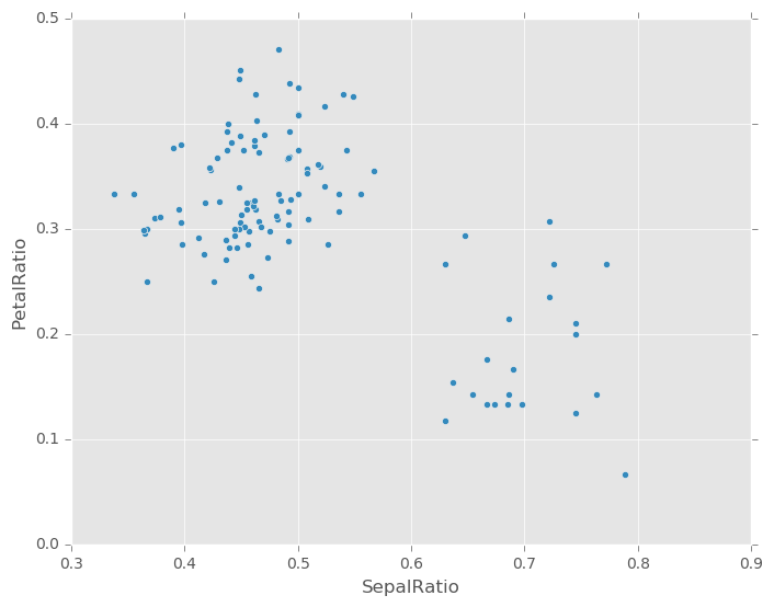
Since a function is passed in, the function is computed on the DataFrame being assigned to. Importantly, this is the DataFrame that’s been filtered to those rows with sepal length greater than 5. The filtering happens first, and then the ratio calculations. This is an example where we didn’t have a reference to the filtered DataFrame available.
The function signature for assign is simply **kwargs. The keys
are the column names for the new fields, and the values are either a value
to be inserted (for example, a Series or NumPy array), or a function
of one argument to be called on the DataFrame. A copy of the original
DataFrame is returned, with the new values inserted.
Warning
Since the function signature of assign is **kwargs, a dictionary,
the order of the new columns in the resulting DataFrame cannot be guaranteed
to match the order you pass in. To make things predictable, items are inserted
alphabetically (by key) at the end of the DataFrame.
All expressions are computed first, and then assigned. So you can’t refer
to another column being assigned in the same call to assign. For example:
In [74]: # Don't do this, bad reference to `C`
        df.assign(C = lambda x: x['A'] + x['B'],
                  D = lambda x: x['A'] + x['C'])
In [2]: # Instead, break it into two assigns
        (df.assign(C = lambda x: x['A'] + x['B'])
           .assign(D = lambda x: x['A'] + x['C']))
Indexing / Selection
The basics of indexing are as follows:
| Operation | Syntax | Result |
|---|---|---|
| Select column | df[col] |
Series |
| Select row by label | df.loc[label] |
Series |
| Select row by integer location | df.iloc[loc] |
Series |
| Slice rows | df[5:10] |
DataFrame |
| Select rows by boolean vector | df[bool_vec] |
DataFrame |
Row selection, for example, returns a Series whose index is the columns of the DataFrame:
In [75]: df.loc['b']
Out[75]:
one 2
bar 2
flag False
foo bar
one_trunc 2
Name: b, dtype: object
In [76]: df.iloc[2]
��������������������������������������������������������������������������������������������������������������������������������Out[76]:
one 3
bar 3
flag True
foo bar
one_trunc NaN
Name: c, dtype: object
For a more exhaustive treatment of more sophisticated label-based indexing and slicing, see the section on indexing. We will address the fundamentals of reindexing / conforming to new sets of labels in the section on reindexing.
Data alignment and arithmetic
Data alignment between DataFrame objects automatically align on both the columns and the index (row labels). Again, the resulting object will have the union of the column and row labels.
In [77]: df = pd.DataFrame(np.random.randn(10, 4), columns=['A', 'B', 'C', 'D'])

In [78]: df2 = pd.DataFrame(np.random.randn(7, 3), columns=['A', 'B', 'C'])

In [79]: df + df2
Out[79]:
        A       B       C   D
0  1.3073  2.4946  0.9907 NaN
1  2.5226 -0.0380 -0.6179 NaN
2 -0.1333 -1.4784 -0.5667 NaN
3 -0.4633 -0.6815  1.5152 NaN
4  0.0622 -1.1679  0.5534 NaN
5  3.1876 -0.0249  0.6607 NaN
6 -0.8777 -0.0846 -2.7677 NaN
7     NaN     NaN     NaN NaN
8     NaN     NaN     NaN NaN
9     NaN     NaN     NaN NaN
When doing an operation between DataFrame and Series, the default behavior is to align the Series index on the DataFrame columns, thus broadcasting row-wise. For example:
In [80]: df - df.iloc[0]
Out[80]:
        A       B       C       D
0  0.0000  0.0000  0.0000  0.0000
1  0.6956 -0.9760 -0.5268 -0.4261
2 -0.6277 -1.9284 -1.7718  3.4021
3 -0.4289 -1.1245 -0.0013  2.2955
4  0.6241 -1.9643 -0.6090  2.0827
5  0.7796  0.0866 -0.2222  2.6553
6  0.1325 -1.4229 -2.2840 -0.0538
7 -0.3135 -1.9574 -0.5461  3.3179
8  0.6366 -1.2767 -0.4022  1.6091
9 -2.4500 -1.5917 -1.0151  3.1963
In the special case of working with time series data, and the DataFrame index also contains dates, the broadcasting will be column-wise:
In [81]: index = pd.date_range('1/1/2000', periods=8)
In [82]: df = pd.DataFrame(np.random.randn(8, 3), index=index, columns=list('ABC'))
In [83]: df
Out[83]:
A B C
2000-01-01 -0.0817 1.3905 -1.9620
2000-01-02 -0.5056 0.0213 -0.3171
2000-01-03 -0.0259 0.8407 1.4135
2000-01-04 0.0492 0.4879 0.4263
2000-01-05 1.2432 -0.6222 -0.5386
2000-01-06 0.7915 -0.0203 0.1844
2000-01-07 -0.1616 0.6414 -1.8116
2000-01-08 -0.1140 -0.8574 0.1719
In [84]: type(df['A'])
�������������������������������������������������������������������������������������������������������������������������������������������������������������������������������������������������������������������������������������������������������������������������������������������������������������������������������������Out[84]: pandas.core.series.Series
In [85]: df - df['A']
������������������������������������������������������������������������������������������������������������������������������������������������������������������������������������������������������������������������������������������������������������������������������������������������������������������������������������������������������������������������Out[85]:
2000-01-01 00:00:00 2000-01-02 00:00:00 2000-01-03 00:00:00 \
2000-01-01 NaN NaN NaN
2000-01-02 NaN NaN NaN
2000-01-03 NaN NaN NaN
2000-01-04 NaN NaN NaN
2000-01-05 NaN NaN NaN
2000-01-06 NaN NaN NaN
2000-01-07 NaN NaN NaN
2000-01-08 NaN NaN NaN
2000-01-04 00:00:00 ... 2000-01-08 00:00:00 A B C
2000-01-01 NaN ... NaN NaN NaN NaN
2000-01-02 NaN ... NaN NaN NaN NaN
2000-01-03 NaN ... NaN NaN NaN NaN
2000-01-04 NaN ... NaN NaN NaN NaN
2000-01-05 NaN ... NaN NaN NaN NaN
2000-01-06 NaN ... NaN NaN NaN NaN
2000-01-07 NaN ... NaN NaN NaN NaN
2000-01-08 NaN ... NaN NaN NaN NaN
[8 rows x 11 columns]
Warning
df - df['A']
is now deprecated and will be removed in a future release. The preferred way to replicate this behavior is
df.sub(df['A'], axis=0)
For explicit control over the matching and broadcasting behavior, see the section on flexible binary operations.
Operations with scalars are just as you would expect:
In [86]: df * 5 + 2
Out[86]:
A B C
2000-01-01 1.5914 8.9525 -7.8102
2000-01-02 -0.5279 2.1063 0.4146
2000-01-03 1.8705 6.2037 9.0676
2000-01-04 2.2461 4.4393 4.1314
2000-01-05 8.2159 -1.1111 -0.6930
2000-01-06 5.9576 1.8985 2.9221
2000-01-07 1.1918 5.2071 -7.0578
2000-01-08 1.4298 -2.2869 2.8595
In [87]: 1 / df
�������������������������������������������������������������������������������������������������������������������������������������������������������������������������������������������������������������������������������������������������������������������������������������������������������������������������������������Out[87]:
A B C
2000-01-01 -12.2384 0.7192 -0.5097
2000-01-02 -1.9779 47.0519 -3.1539
2000-01-03 -38.6178 1.1894 0.7075
2000-01-04 20.3130 2.0498 2.3458
2000-01-05 0.8044 -1.6072 -1.8566
2000-01-06 1.2634 -49.2551 5.4221
2000-01-07 -6.1864 1.5590 -0.5520
2000-01-08 -8.7695 -1.1663 5.8170
In [88]: df ** 4
��������������������������������������������������������������������������������������������������������������������������������������������������������������������������������������������������������������������������������������������������������������������������������������������������������������������������������������������������������������������������������������������������������������������������������������������������������������������������������������������������������������������������������������������������������������������������������������������������������������������������������������������������������������������������������������������Out[88]:
A B C
2000-01-01 4.4576e-05 3.7384e+00 14.8192
2000-01-02 6.5337e-02 2.0403e-07 0.0101
2000-01-03 4.4962e-07 4.9964e-01 3.9922
2000-01-04 5.8735e-06 5.6645e-02 0.0330
2000-01-05 2.3885e+00 1.4989e-01 0.0842
2000-01-06 3.9249e-01 1.6990e-07 0.0012
2000-01-07 6.8273e-04 1.6926e-01 10.7700
2000-01-08 1.6908e-04 5.4038e-01 0.0009
Boolean operators work as well:
In [89]: df1 = pd.DataFrame({'a' : [1, 0, 1], 'b' : [0, 1, 1] }, dtype=bool)
In [90]: df2 = pd.DataFrame({'a' : [0, 1, 1], 'b' : [1, 1, 0] }, dtype=bool)
In [91]: df1 & df2
Out[91]:
a b
0 False False
1 False True
2 True False
In [92]: df1 | df2
��������������������������������������������������������������������������Out[92]:
a b
0 True True
1 True True
2 True True
In [93]: df1 ^ df2
��������������������������������������������������������������������������������������������������������������������������������������������Out[93]:
a b
0 True True
1 True False
2 False True
In [94]: -df1
����������������������������������������������������������������������������������������������������������������������������������������������������������������������������������������������������������������������Out[94]:
a b
0 False True
1 True False
2 False False
Transposing
To transpose, access the T attribute (also the transpose function),
similar to an ndarray:
# only show the first 5 rows
In [95]: df[:5].T
Out[95]:
   2000-01-01  2000-01-02  2000-01-03  2000-01-04  2000-01-05
A     -0.0817     -0.5056     -0.0259      0.0492      1.2432
B      1.3905      0.0213      0.8407      0.4879     -0.6222
C     -1.9620     -0.3171      1.4135      0.4263     -0.5386
DataFrame interoperability with NumPy functions
Elementwise NumPy ufuncs (log, exp, sqrt, ...) and various other NumPy functions can be used with no issues on DataFrame, assuming the data within are numeric:
In [96]: np.exp(df)
Out[96]:
A B C
2000-01-01 0.9215 4.0169 0.1406
2000-01-02 0.6032 1.0215 0.7283
2000-01-03 0.9744 2.3181 4.1104
2000-01-04 1.0505 1.6288 1.5316
2000-01-05 3.4666 0.5368 0.5836
2000-01-06 2.2067 0.9799 1.2025
2000-01-07 0.8507 1.8992 0.1634
2000-01-08 0.8922 0.4243 1.1876
In [97]: np.asarray(df)
�������������������������������������������������������������������������������������������������������������������������������������������������������������������������������������������������������������������������������������������������������������������������������������������������������������������������������������Out[97]:
array([[-0.0817, 1.3905, -1.962 ],
[-0.5056, 0.0213, -0.3171],
[-0.0259, 0.8407, 1.4135],
[ 0.0492, 0.4879, 0.4263],
[ 1.2432, -0.6222, -0.5386],
[ 0.7915, -0.0203, 0.1844],
[-0.1616, 0.6414, -1.8116],
[-0.114 , -0.8574, 0.1719]])
The dot method on DataFrame implements matrix multiplication:
In [98]: df.T.dot(df)
Out[98]:
        A       B       C
A  2.4765 -0.9176  0.0546
B -0.9176  4.4129 -2.3166
C  0.0546 -2.3166  9.7653
Similarly, the dot method on Series implements dot product:
In [99]: s1 = pd.Series(np.arange(5,10))

In [100]: s1.dot(s1)
Out[100]: 255
DataFrame is not intended to be a drop-in replacement for ndarray as its indexing semantics are quite different in places from a matrix.
Console display
Very large DataFrames will be truncated to display them in the console.
You can also get a summary using info().
(Here I am reading a CSV version of the baseball dataset from the plyr
R package):
In [101]: baseball = pd.read_csv('data/baseball.csv')
In [102]: print(baseball)
id player year stint ... hbp sh sf gidp
0 88641 womacto01 2006 2 ... 0.0 3.0 0.0 0.0
1 88643 schilcu01 2006 1 ... 0.0 0.0 0.0 0.0
.. ... ... ... ... ... ... ... ... ...
98 89533 aloumo01 2007 1 ... 2.0 0.0 3.0 13.0
99 89534 alomasa02 2007 1 ... 0.0 0.0 0.0 0.0
[100 rows x 23 columns]
In [103]: baseball.info()
�������������������������������������������������������������������������������������������������������������������������������������������������������������������������������������������������������������������������������������������������������������������������������������������������������������������������������������������������������������������������������������������������������<class 'pandas.core.frame.DataFrame'>
RangeIndex: 100 entries, 0 to 99
Data columns (total 23 columns):
id 100 non-null int64
player 100 non-null object
year 100 non-null int64
stint 100 non-null int64
team 100 non-null object
lg 100 non-null object
g 100 non-null int64
ab 100 non-null int64
r 100 non-null int64
h 100 non-null int64
X2b 100 non-null int64
X3b 100 non-null int64
hr 100 non-null int64
rbi 100 non-null float64
sb 100 non-null float64
cs 100 non-null float64
bb 100 non-null int64
so 100 non-null float64
ibb 100 non-null float64
hbp 100 non-null float64
sh 100 non-null float64
sf 100 non-null float64
gidp 100 non-null float64
dtypes: float64(9), int64(11), object(3)
memory usage: 18.0+ KB
However, using to_string will return a string representation of the
DataFrame in tabular form, though it won’t always fit the console width:
In [104]: print(baseball.iloc[-20:, :12].to_string())
       id     player  year  stint team  lg    g   ab   r    h  X2b  X3b
80  89474  finlest01  2007      1  COL  NL   43   94   9   17    3    0
81  89480  embreal01  2007      1  OAK  AL    4    0   0    0    0    0
82  89481  edmonji01  2007      1  SLN  NL  117  365  39   92   15    2
83  89482  easleda01  2007      1  NYN  NL   76  193  24   54    6    0
84  89489  delgaca01  2007      1  NYN  NL  139  538  71  139   30    0
85  89493  cormirh01  2007      1  CIN  NL    6    0   0    0    0    0
86  89494  coninje01  2007      2  NYN  NL   21   41   2    8    2    0
87  89495  coninje01  2007      1  CIN  NL   80  215  23   57   11    1
88  89497  clemero02  2007      1  NYA  AL    2    2   0    1    0    0
89  89498  claytro01  2007      2  BOS  AL    8    6   1    0    0    0
90  89499  claytro01  2007      1  TOR  AL   69  189  23   48   14    0
91  89501  cirilje01  2007      2  ARI  NL   28   40   6    8    4    0
92  89502  cirilje01  2007      1  MIN  AL   50  153  18   40    9    2
93  89521  bondsba01  2007      1  SFN  NL  126  340  75   94   14    0
94  89523  biggicr01  2007      1  HOU  NL  141  517  68  130   31    3
95  89525  benitar01  2007      2  FLO  NL   34    0   0    0    0    0
96  89526  benitar01  2007      1  SFN  NL   19    0   0    0    0    0
97  89530  ausmubr01  2007      1  HOU  NL  117  349  38   82   16    3
98  89533   aloumo01  2007      1  NYN  NL   87  328  51  112   19    1
99  89534  alomasa02  2007      1  NYN  NL    8   22   1    3    1    0
New since 0.10.0, wide DataFrames will now be printed across multiple rows by default:
In [105]: pd.DataFrame(np.random.randn(3, 12))
Out[105]:
         0         1         2         3         4         5         6   \
0 -1.040542 -1.126415  0.549956  1.323044 -0.219197  0.581467 -0.519407
1 -2.603736  0.532069  0.327184 -1.251625  1.481966 -0.642683  1.248002
2  0.683625 -1.876826 -1.873827 -0.251457  0.027599  1.235291  0.850574

         7         8         9         10        11
0 -0.271582  0.344684 -0.643988 -0.378918 -0.924127
1  1.954333 -0.475215 -1.258974 -1.142863 -1.015321
2 -1.140302  2.149143  0.504452  0.678026 -0.628443
You can change how much to print on a single row by setting the display.width
option:
In [106]: pd.set_option('display.width', 40) # default is 80

In [107]: pd.DataFrame(np.random.randn(3, 12))
Out[107]:
         0         1         2   \
0  1.191156 -1.145363 -0.523153
1  0.762474  0.481666  1.217546
2  0.076257 -0.897159 -1.265679

         3         4         5   \
0 -1.299878 -0.110240 -0.333712
1  0.577103 -0.076021  0.720235
2 -0.528311 -0.660014 -0.117339

         6         7         8   \
0  0.416876 -0.436400  0.999768
1  0.202660 -0.314950 -0.410852
2  0.780048  2.162047  0.874233

         9         10        11
0 -0.383171 -0.172217 -1.674685
1  0.542758  1.955407 -0.940645
2 -0.764147 -0.484495  0.298570
You can adjust the max width of the individual columns by setting display.max_colwidth
In [108]: datafile={'filename': ['filename_01','filename_02'],
   .....:           'path': ["media/user_name/storage/folder_01/filename_01",
   .....:                    "media/user_name/storage/folder_02/filename_02"]}
   .....:

In [109]: pd.set_option('display.max_colwidth',30)

In [110]: pd.DataFrame(datafile)
Out[110]:
      filename  \
0  filename_01
1  filename_02

                            path
0  media/user_name/storage/fo...
1  media/user_name/storage/fo...

In [111]: pd.set_option('display.max_colwidth',100)

In [112]: pd.DataFrame(datafile)
Out[112]:
      filename  \
0  filename_01
1  filename_02

                                            path
0  media/user_name/storage/folder_01/filename_01
1  media/user_name/storage/folder_02/filename_02
You can also disable this feature via the expand_frame_repr option.
This will print the table in one block.
DataFrame column attribute access and IPython completion
If a DataFrame column label is a valid Python variable name, the column can be accessed like attributes:
In [113]: df = pd.DataFrame({'foo1' : np.random.randn(5),
.....: 'foo2' : np.random.randn(5)})
.....:
In [114]: df
Out[114]:
foo1 foo2
0 0.825136 -1.749969
1 -0.388020 -1.402941
2 -0.339279 0.623222
3 0.141164 0.020129
4 0.565930 -2.858463
In [115]: df.foo1
�����������������������������������������������������������������������������������������������������������������������������������������������Out[115]:
0 0.825136
1 -0.388020
2 -0.339279
3 0.141164
4 0.565930
Name: foo1, dtype: float64
The columns are also connected to the IPython completion mechanism so they can be tab-completed:
In [5]: df.fo<TAB>
df.foo1  df.foo2
Panel
Warning
In 0.20.0, Panel is deprecated and will be removed in
a future version. See the section Deprecate Panel.
Panel is a somewhat less-used, but still important container for 3-dimensional data. The term panel data is derived from econometrics and is partially responsible for the name pandas: pan(el)-da(ta)-s. The names for the 3 axes are intended to give some semantic meaning to describing operations involving panel data and, in particular, econometric analysis of panel data. However, for the strict purposes of slicing and dicing a collection of DataFrame objects, you may find the axis names slightly arbitrary:
- items: axis 0, each item corresponds to a DataFrame contained inside
- major_axis: axis 1, it is the index (rows) of each of the DataFrames
- minor_axis: axis 2, it is the columns of each of the DataFrames
Construction of Panels works about like you would expect:
From 3D ndarray with optional axis labels
In [116]: wp = pd.Panel(np.random.randn(2, 5, 4), items=['Item1', 'Item2'],
   .....:               major_axis=pd.date_range('1/1/2000', periods=5),
   .....:               minor_axis=['A', 'B', 'C', 'D'])
   .....:

In [117]: wp
Out[117]:
<class 'pandas.core.panel.Panel'>
Dimensions: 2 (items) x 5 (major_axis) x 4 (minor_axis)
Items axis: Item1 to Item2
Major_axis axis: 2000-01-01 00:00:00 to 2000-01-05 00:00:00
Minor_axis axis: A to D
From dict of DataFrame objects
In [118]: data = {'Item1' : pd.DataFrame(np.random.randn(4, 3)),
   .....:         'Item2' : pd.DataFrame(np.random.randn(4, 2))}
   .....:

In [119]: pd.Panel(data)
Out[119]:
<class 'pandas.core.panel.Panel'>
Dimensions: 2 (items) x 4 (major_axis) x 3 (minor_axis)
Items axis: Item1 to Item2
Major_axis axis: 0 to 3
Minor_axis axis: 0 to 2
Note that the values in the dict need only be convertible to DataFrame. Thus, they can be any of the other valid inputs to DataFrame as per above.
One helpful factory method is Panel.from_dict, which takes a
dictionary of DataFrames as above, and the following named parameters:
| Parameter | Default | Description |
|---|---|---|
| intersect | False |
drops elements whose indices do not align |
| orient | items |
use minor to use DataFrames’ columns as panel items |
For example, compare to the construction above:
In [120]: pd.Panel.from_dict(data, orient='minor')
Out[120]:
<class 'pandas.core.panel.Panel'>
Dimensions: 3 (items) x 4 (major_axis) x 2 (minor_axis)
Items axis: 0 to 2
Major_axis axis: 0 to 3
Minor_axis axis: Item1 to Item2
Orient is especially useful for mixed-type DataFrames. If you pass a dict of
DataFrame objects with mixed-type columns, all of the data will get upcasted to
dtype=object unless you pass orient='minor':
In [121]: df = pd.DataFrame({'a': ['foo', 'bar', 'baz'],
.....: 'b': np.random.randn(3)})
.....:
In [122]: df
Out[122]:
a b
0 foo 1.047583
1 bar 0.507575
2 baz 1.172740
In [123]: data = {'item1': df, 'item2': df}
In [124]: panel = pd.Panel.from_dict(data, orient='minor')
In [125]: panel['a']
Out[125]:
item1 item2
0 foo foo
1 bar bar
2 baz baz
In [126]: panel['b']
�������������������������������������������������������������������Out[126]:
item1 item2
0 1.047583 1.047583
1 0.507575 0.507575
2 1.172740 1.172740
In [127]: panel['b'].dtypes
����������������������������������������������������������������������������������������������������������������������������������������������������������������������Out[127]:
item1 float64
item2 float64
dtype: object
Note
Unfortunately Panel, being less commonly used than Series and DataFrame, has been slightly neglected feature-wise. A number of methods and options available in DataFrame are not available in Panel. This will get worked on, of course, in future releases. And faster if you join me in working on the codebase.
From DataFrame using to_panel method
This method was introduced in v0.7 to replace LongPanel.to_long, and converts
a DataFrame with a two-level index to a Panel.
In [128]: midx = pd.MultiIndex(levels=[['one', 'two'], ['x','y']], labels=[[1,1,0,0],[1,0,1,0]])

In [129]: df = pd.DataFrame({'A' : [1, 2, 3, 4], 'B': [5, 6, 7, 8]}, index=midx)

In [130]: df.to_panel()
Out[130]:
<class 'pandas.core.panel.Panel'>
Dimensions: 2 (items) x 2 (major_axis) x 2 (minor_axis)
Items axis: A to B
Major_axis axis: one to two
Minor_axis axis: x to y
Item selection / addition / deletion
Similar to DataFrame functioning as a dict of Series, Panel is like a dict of DataFrames:
In [131]: wp['Item1']
Out[131]:
                   A         B         C         D
2000-01-01  0.885765  0.158014 -1.981797  1.769622
2000-01-02  0.093792 -1.269228  1.290159  0.509707
2000-01-03 -0.251960 -1.127396 -0.430936 -1.243710
2000-01-04 -0.854956 -0.327742  0.210942  0.152473
2000-01-05 -0.061545  2.845263 -0.507224  1.772662

In [132]: wp['Item3'] = wp['Item1'] / wp['Item2']
The API for insertion and deletion is the same as for DataFrame. And as with DataFrame, if the item is a valid python identifier, you can access it as an attribute and tab-complete it in IPython.
Transposing
A Panel can be rearranged using its transpose method (which does not make a
copy by default unless the data are heterogeneous):
In [133]: wp.transpose(2, 0, 1)
Out[133]:
<class 'pandas.core.panel.Panel'>
Dimensions: 4 (items) x 3 (major_axis) x 5 (minor_axis)
Items axis: A to D
Major_axis axis: Item1 to Item3
Minor_axis axis: 2000-01-01 00:00:00 to 2000-01-05 00:00:00
Indexing / Selection
| Operation | Syntax | Result |
|---|---|---|
| Select item | wp[item] |
DataFrame |
| Get slice at major_axis label | wp.major_xs(val) |
DataFrame |
| Get slice at minor_axis label | wp.minor_xs(val) |
DataFrame |
For example, using the earlier example data, we could do:
In [134]: wp['Item1']
Out[134]:
A B C D
2000-01-01 0.885765 0.158014 -1.981797 1.769622
2000-01-02 0.093792 -1.269228 1.290159 0.509707
2000-01-03 -0.251960 -1.127396 -0.430936 -1.243710
2000-01-04 -0.854956 -0.327742 0.210942 0.152473
2000-01-05 -0.061545 2.845263 -0.507224 1.772662
In [135]: wp.major_xs(wp.major_axis[2])
�����������������������������������������������������������������������������������������������������������������������������������������������������������������������������������������������������������������������������������������������������������������������������������������������������������������������������Out[135]:
Item1 Item2 Item3
A -0.251960 -0.107412 2.345742
B -1.127396 0.765200 -1.473335
C -0.430936 0.387271 -1.112751
D -1.243710 1.456602 -0.853843
In [136]: wp.minor_axis
��������������������������������������������������������������������������������������������������������������������������������������������������������������������������������������������������������������������������������������������������������������������������������������������������������������������������������������������������������������������������������������������������������������������������������������������������������������������������������������������������������Out[136]: Index(['A', 'B', 'C', 'D'], dtype='object')
In [137]: wp.minor_xs('C')
��������������������������������������������������������������������������������������������������������������������������������������������������������������������������������������������������������������������������������������������������������������������������������������������������������������������������������������������������������������������������������������������������������������������������������������������������������������������������������������������������������������������������������������������������������������Out[137]:
Item1 Item2 Item3
2000-01-01 -1.981797 0.821163 -2.413403
2000-01-02 1.290159 0.037155 34.724047
2000-01-03 -0.430936 0.387271 -1.112751
2000-01-04 0.210942 -0.016899 -12.482295
2000-01-05 -0.507224 1.760286 -0.288149
Squeezing
Another way to change the dimensionality of an object is to squeeze a 1-len object, similar to wp['Item1']
In [138]: wp.reindex(items=['Item1']).squeeze()
Out[138]:
A B C D
2000-01-01 0.885765 0.158014 -1.981797 1.769622
2000-01-02 0.093792 -1.269228 1.290159 0.509707
2000-01-03 -0.251960 -1.127396 -0.430936 -1.243710
2000-01-04 -0.854956 -0.327742 0.210942 0.152473
2000-01-05 -0.061545 2.845263 -0.507224 1.772662
In [139]: wp.reindex(items=['Item1'], minor=['B']).squeeze()
�����������������������������������������������������������������������������������������������������������������������������������������������������������������������������������������������������������������������������������������������������������������������������������������������������������������������������Out[139]:
2000-01-01 0.158014
2000-01-02 -1.269228
2000-01-03 -1.127396
2000-01-04 -0.327742
2000-01-05 2.845263
Freq: D, Name: B, dtype: float64
Conversion to DataFrame
A Panel can be represented in 2D form as a hierarchically indexed
DataFrame. See the section hierarchical indexing
for more on this. To convert a Panel to a DataFrame, use the to_frame
method:
In [140]: panel = pd.Panel(np.random.randn(3, 5, 4), items=['one', 'two', 'three'],
   .....:                  major_axis=pd.date_range('1/1/2000', periods=5),
   .....:                  minor_axis=['a', 'b', 'c', 'd'])
   .....:

In [141]: panel.to_frame()
Out[141]:
                       one       two     three
major      minor
2000-01-01 a      0.368964 -2.033050  0.525741
           b     -1.596338 -0.271503  1.311232
           c      0.294397  0.000658  0.535689
           d      1.633316  0.301351  0.350587
2000-01-02 a      0.613334 -0.977983 -0.691015
           b     -0.561237 -0.310997  0.893930
           c     -1.316660  0.608487  2.064058
           d      1.038137  1.791018  0.548489
2000-01-03 a     -1.367749 -0.724384 -1.298233
           b      0.010581  0.327463 -0.286955
           c      0.882541 -1.046022 -0.193618
           d      0.177449 -1.424694  1.122169
2000-01-04 a      0.291669  1.845002  1.289298
           b      2.177649  0.099995 -0.811164
           c      0.741563  0.368960 -0.902172
           d      0.524001 -0.025353 -0.093062
2000-01-05 a     -1.154972  0.635333  0.687572
           b     -2.075966 -1.484139 -0.653155
           c     -0.858758  0.259096 -1.321267
           d     -0.868204  0.817009 -0.593775
Deprecate Panel
Over the last few years, pandas has increased in both breadth and depth, with new features,
datatype support, and manipulation routines. As a result, supporting efficient indexing and functional
routines for Series, DataFrame and Panel has contributed to an increasingly fragmented and
difficult-to-understand codebase.
The 3-D structure of a Panel is much less common for many types of data analysis,
than the 1-D of the Series or the 2-D of the DataFrame. Going forward it makes sense for
pandas to focus on these areas exclusively.
Oftentimes, one can simply use a MultiIndex DataFrame for easily working with higher dimensional data.
In additon, the xarray package was built from the ground up, specifically in order to
support the multi-dimensional analysis that is one of Panel s main usecases.
Here is a link to the xarray panel-transition documentation.
In [142]: p = tm.makePanel()

In [143]: p
Out[143]:
<class 'pandas.core.panel.Panel'>
Dimensions: 3 (items) x 30 (major_axis) x 4 (minor_axis)
Items axis: ItemA to ItemC
Major_axis axis: 2000-01-03 00:00:00 to 2000-02-11 00:00:00
Minor_axis axis: A to D
Convert to a MultiIndex DataFrame
In [144]: p.to_frame()
Out[144]:
                     ItemA     ItemB     ItemC
major      minor
2000-01-03 A     -0.562101  0.596722 -0.006076
           B     -1.188433  0.623781  0.414700
           C     -1.122897  1.570412 -1.121722
           D      1.068153  0.637637 -0.332359
2000-01-04 A      0.348637 -1.196606  0.584980
           B     -0.364369  0.044965 -0.104393
           C      1.255063 -1.555786  1.864044
           D      0.645839 -1.004495  0.211849
2000-01-05 A     -3.136335  0.684902  0.764032
           B     -0.522007 -0.700244  0.618741
           C      1.019730  1.515842 -1.117555
           D      1.966118  1.146482  1.156103
2000-01-06 A      0.950982 -2.420257 -0.334286
           B      0.379510 -0.800428  1.477061
           C     -0.185257  1.535935 -0.459102
           D      1.929061  0.955239 -0.167683
2000-01-07 A     -0.817696 -0.497864  0.723964
           B      0.219003 -0.262461 -0.479880
           C      0.980392  0.440980  0.254221
           D      0.515374  0.393402  1.725259
2000-01-10 A     -1.522532 -1.155281 -1.294066
           B     -1.434896  0.294109 -0.338110
           C      0.363619  0.923475 -0.180491
           D     -0.007877  0.886686 -0.482607
2000-01-11 A      0.877248 -0.182729  1.511304
           B      1.137177  0.455629  0.169672
           C      1.044038 -1.046968  1.634983
           D      0.566788 -0.961336 -0.008121
2000-01-12 A     -0.596688  1.440756  0.917094
           B     -0.004067  0.610660  0.187756
...                    ...       ...       ...
2000-02-02 C     -1.426564 -0.315895 -0.729149
           D     -1.951812  0.298852 -1.409432
2000-02-03 A      0.876211  1.780657  1.232949
           B      0.753136  0.626754  0.480243
           C      0.307062 -0.513063 -1.543837
           D     -0.304052  0.626159 -0.433954
2000-02-04 A     -1.510807 -0.508626  1.396962
           B     -0.453719  0.243984  0.188892
           C      0.846308 -0.000835  0.058163
           D     -0.378778  0.651006 -0.382207
2000-02-07 A      1.178281 -0.319874  0.081011
           B      1.272689  1.471866  0.177015
           C     -0.443532  0.232687  0.050537
           D     -0.363109  0.767951 -0.927974
2000-02-08 A     -0.838111  0.608138  1.055219
           B     -0.449769  0.170149 -1.206715
           C     -0.582117 -0.619567 -0.746344
           D      0.355729  1.179747 -1.684914
2000-02-09 A      0.018222 -0.239844  0.098448
           B     -2.178055 -1.672600  0.210899
           C      1.585616  0.167086  1.079875
           D     -0.931390  0.027154 -0.038714
2000-02-10 A      3.082589  0.418458 -0.202864
           B      0.431345  0.251429  0.264253
           C     -0.108185  0.422885  0.966498
           D      0.928076  1.326783 -0.897329
2000-02-11 A      0.453499  0.655473 -0.287878
           B     -0.279384  0.879678 -0.032215
           C     -0.555896 -0.780570 -1.366063
           D      0.771169  1.339542  0.032964

[120 rows x 3 columns]
Alternatively, one can convert to an xarray DataArray.
In [145]: p.to_xarray()
Out[145]:
<xarray.DataArray (items: 3, major_axis: 30, minor_axis: 4)>
array([[[-0.562101, -1.188433, -1.122897,  1.068153],
        [ 0.348637, -0.364369,  1.255063,  0.645839],
        ...,
        [ 3.082589,  0.431345, -0.108185,  0.928076],
        [ 0.453499, -0.279384, -0.555896,  0.771169]],

       [[ 0.596722,  0.623781,  1.570412,  0.637637],
        [-1.196606,  0.044965, -1.555786, -1.004495],
        ...,
        [ 0.418458,  0.251429,  0.422885,  1.326783],
        [ 0.655473,  0.879678, -0.78057 ,  1.339542]],

       [[-0.006076,  0.4147  , -1.121722, -0.332359],
        [ 0.58498 , -0.104393,  1.864044,  0.211849],
        ...,
        [-0.202864,  0.264253,  0.966498, -0.897329],
        [-0.287878, -0.032215, -1.366063,  0.032964]]])
Coordinates:
  * items       (items) object 'ItemA' 'ItemB' 'ItemC'
  * major_axis  (major_axis) datetime64[ns] 2000-01-03 2000-01-04 2000-01-05 ...
  * minor_axis  (minor_axis) object 'A' 'B' 'C' 'D'
You can see the full-documentation for the xarray package.
Panel4D and PanelND (Deprecated)
Warning
In 0.19.0 Panel4D and PanelND are deprecated and will be removed in
a future version. The recommended way to represent these types of
n-dimensional data are with the
xarray package.
Pandas provides a to_xarray() method to automate
this conversion.
See the docs of a previous version for documentation on these objects.