Computational tools¶

Statistical functions¶

Covariance¶

The Series object has a method cov to compute covariance between series (excluding NA/null values).

In [157]: s1 = Series(randn(1000))

In [158]: s2 = Series(randn(1000))

In [159]: s1.cov(s2)
Out[159]: 0.019465636696791695

Analogously, DataFrame has a method cov to compute pairwise covariances among the series in the DataFrame, also excluding NA/null values.

In [160]: frame = DataFrame(randn(1000, 5), columns=['a', 'b', 'c', 'd', 'e'])

In [161]: frame.cov()
Out[161]: 
          a         b         c         d         e
a  0.953751 -0.029550 -0.006415  0.001020 -0.004134
b -0.029550  0.997223 -0.044276  0.005967  0.044884
c -0.006415 -0.044276  1.050236  0.077775  0.010642
d  0.001020  0.005967  0.077775  0.998485 -0.007345
e -0.004134  0.044884  0.010642 -0.007345  1.025446

Correlation¶

Several methods for computing correlations are provided. Several kinds of correlation methods are provided:

Method name	Description
`pearson (default)`	Standard correlation coefficient
`kendall`	Kendall Tau correlation coefficient
`spearman`	Spearman rank correlation coefficient

All of these are currently computed using pairwise complete observations.

In [162]: frame = DataFrame(randn(1000, 5), columns=['a', 'b', 'c', 'd', 'e'])

In [163]: frame.ix[::2] = np.nan

# Series with Series
In [164]: frame['a'].corr(frame['b'])
Out[164]: 0.013306883832198543

In [165]: frame['a'].corr(frame['b'], method='spearman')
Out[165]: 0.022530330121320486

# Pairwise correlation of DataFrame columns
In [166]: frame.corr()
Out[166]: 
          a         b         c         d         e
a  1.000000  0.013307 -0.037801 -0.021905  0.001165
b  0.013307  1.000000 -0.017259  0.079246 -0.043606
c -0.037801 -0.017259  1.000000  0.061657  0.078945
d -0.021905  0.079246  0.061657  1.000000 -0.036978
e  0.001165 -0.043606  0.078945 -0.036978  1.000000

Note that non-numeric columns will be automatically excluded from the correlation calculation.

A related method corrwith is implemented on DataFrame to compute the correlation between like-labeled Series contained in different DataFrame objects.

In [167]: index = ['a', 'b', 'c', 'd', 'e']

In [168]: columns = ['one', 'two', 'three', 'four']

In [169]: df1 = DataFrame(randn(5, 4), index=index, columns=columns)

In [170]: df2 = DataFrame(randn(4, 4), index=index[:4], columns=columns)

In [171]: df1.corrwith(df2)
Out[171]: 
one      0.344149
two      0.837438
three    0.458904
four     0.712401

In [172]: df2.corrwith(df1, axis=1)
Out[172]: 
a    0.404019
b    0.772204
c    0.420390
d   -0.142959
e         NaN

Data ranking¶

The rank method produces a data ranking with ties being assigned the mean of the ranks (by default) for the group:

In [173]: s = Series(np.random.randn(5), index=list('abcde'))

In [174]: s['d'] = s['b'] # so there's a tie

In [175]: s.rank()
Out[175]: 
a    2.0
b    3.5
c    1.0
d    3.5
e    5.0

rank is also a DataFrame method and can rank either the rows (axis=0) or the columns (axis=1). NaN values are excluded from the ranking.

In [176]: df = DataFrame(np.random.randn(10, 6))

In [177]: df[4] = df[2][:5] # some ties

In [178]: df
Out[178]: 
          0         1         2         3         4         5
0.106333  0.712162 -0.351275  1.176287 -0.351275  1.741787
-1.301869  0.612432 -0.577677  0.124709 -0.577677 -1.068084
-0.899627  0.822023  1.506319  0.998896  1.506319  0.259080
-0.522705 -1.473680 -1.726800  1.555343 -1.726800 -1.411978
0.733147  0.415881 -0.026973  0.999488 -0.026973  0.082219
0.995001 -1.399355  0.082244 -1.521795       NaN  0.416180
-0.779714 -0.226893  0.956567 -0.443664       NaN -0.610675
-0.635495 -0.621647  0.406259 -0.279002       NaN -1.153000
0.085011 -0.459422 -1.660917 -1.913019       NaN  0.833479
-0.557052  0.775425  0.003794  0.555351       NaN -1.169977

In [179]: df.rank(1)
Out[179]: 
1    2  3    4  5
3  4  1.5  5  1.5  6
1  6  3.5  5  3.5  2
1  3  5.5  4  5.5  2
5  3  1.5  6  1.5  4
5  4  1.5  6  1.5  3
5  2  3.0  1  NaN  4
1  4  5.0  3  NaN  2
2  3  5.0  4  NaN  1
4  3  2.0  1  NaN  5
2  5  3.0  4  NaN  1

rank optionally takes a parameter ascending which by default is true; when false, data is reverse-ranked, with larger values assigned a smaller rank.

rank supports different tie-breaking methods, specified with the method parameter:

average : average rank of tied group

min : lowest rank in the group

max : highest rank in the group

first : ranks assigned in the order they appear in the array

Note

These methods are significantly faster (around 10-20x) than scipy.stats.rankdata.

Moving (rolling) statistics / moments¶

For working with time series data, a number of functions are provided for computing common moving or rolling statistics. Among these are count, sum, mean, median, correlation, variance, covariance, standard deviation, skewness, and kurtosis. All of these methods are in the pandas namespace, but otherwise they can be found in pandas.stats.moments.

Function	Description
`rolling_count`	Number of non-null observations
`rolling_sum`	Sum of values
`rolling_mean`	Mean of values
`rolling_median`	Arithmetic median of values
`rolling_min`	Minimum
`rolling_max`	Maximum
`rolling_std`	Unbiased standard deviation
`rolling_var`	Unbiased variance
`rolling_skew`	Unbiased skewness (3rd moment)
`rolling_kurt`	Unbiased kurtosis (4th moment)
`rolling_quantile`	Sample quantile (value at %)
`rolling_apply`	Generic apply
`rolling_cov`	Unbiased covariance (binary)
`rolling_corr`	Correlation (binary)
`rolling_corr_pairwise`	Pairwise correlation of DataFrame columns

Generally these methods all have the same interface. The binary operators (e.g. rolling_corr) take two Series or DataFrames. Otherwise, they all accept the following arguments:

window: size of moving window

min_periods: threshold of non-null data points to require (otherwise result is NA)

time_rule: optionally specify a time rule to pre-conform the data to

These functions can be applied to ndarrays or Series objects:

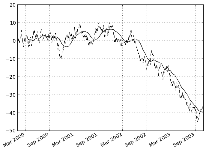
In [180]: ts = Series(randn(1000), index=DateRange('1/1/2000', periods=1000))

In [181]: ts = ts.cumsum()

In [182]: ts.plot(style='k--')
Out[182]: <matplotlib.axes.AxesSubplot at 0x10a7bd6d0>

In [183]: rolling_mean(ts, 60).plot(style='k')
Out[183]: <matplotlib.axes.AxesSubplot at 0x10a7bd6d0>

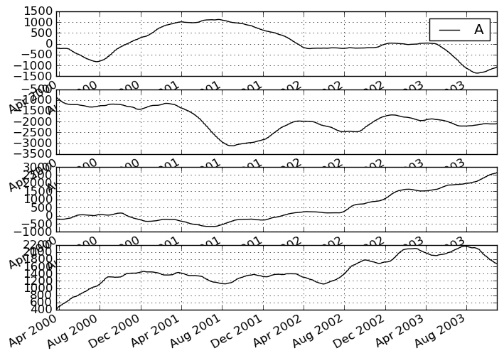
They can also be applied to DataFrame objects. This is really just syntactic sugar for applying the moving window operator to all of the DataFrame’s columns:

In [184]: df = DataFrame(randn(1000, 4), index=ts.index,
   .....:                columns=['A', 'B', 'C', 'D'])

In [185]: df = df.cumsum()

In [186]: rolling_sum(df, 60).plot(subplots=True)
Out[186]: 
array([Axes(0.125,0.747826;0.775x0.152174),
       Axes(0.125,0.565217;0.775x0.152174),
       Axes(0.125,0.382609;0.775x0.152174), Axes(0.125,0.2;0.775x0.152174)], dtype=object)

Binary rolling moments¶

rolling_cov and rolling_corr can compute moving window statistics about two Series or any combination of DataFrame/Series or DataFrame/DataFrame. Here is the behavior in each case:

two Series: compute the statistic for the pairing
DataFrame/Series: compute the statistics for each column of the DataFrame with the passed Series, thus returning a DataFrame
DataFrame/DataFrame: compute statistic for matching column names, returning a DataFrame

For example:

In [187]: df2 = df[:20]

In [188]: rolling_corr(df2, df2['B'], window=5)
Out[188]: 
                   A   B         C         D
2000-01-03       NaN NaN       NaN       NaN
2000-01-04       NaN NaN       NaN       NaN
2000-01-05       NaN NaN       NaN       NaN
2000-01-06       NaN NaN       NaN       NaN
2000-01-07  0.806980   1 -0.911973 -0.747745
2000-01-10  0.689915   1 -0.609054 -0.680394
2000-01-11  0.211679   1 -0.383565 -0.164879
2000-01-12  0.286270   1  0.104075  0.345844
2000-01-13 -0.565249   1  0.039148  0.333921
2000-01-14  0.295310   1  0.501143 -0.524100
2000-01-17  0.041252   1  0.868636 -0.577590
2000-01-18  0.205705   1  0.917778 -0.819271
2000-01-19  0.326449   1  0.933352 -0.882750
2000-01-20  0.120893   1  0.409255 -0.795062
2000-01-21  0.680531   1 -0.192045 -0.349044
2000-01-24  0.643667   1 -0.588676  0.473287
2000-01-25  0.703188   1 -0.746130  0.714265
2000-01-26  0.065322   1 -0.209789  0.635360
2000-01-27 -0.429914   1 -0.100807  0.266005
2000-01-28 -0.387498   1  0.512321  0.592033

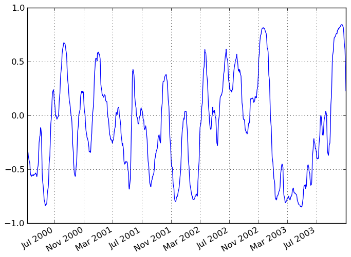
Computing rolling pairwise correlations¶

In financial data analysis and other fields it’s common to compute correlation matrices for a collection of time series. More difficult is to compute a moving-window correlation matrix. This can be done using the rolling_corr_pairwise function, which yields a Panel whose items are the dates in question:

In [189]: correls = rolling_corr_pairwise(df, 50)

In [190]: correls[df.index[-50]]
Out[190]: 
          A         B         C         D
A  1.000000 -0.177708 -0.253742  0.303872
B -0.177708  1.000000 -0.085484  0.008572
C -0.253742 -0.085484  1.000000 -0.769233
D  0.303872  0.008572 -0.769233  1.000000

You can efficiently retrieve the time series of correlations between two columns using ix indexing:

In [191]: correls.ix[:, 'A', 'C'].plot()
Out[191]: <matplotlib.axes.AxesSubplot at 0x10a7bd950>

Exponentially weighted moment functions¶

A related set of functions are exponentially weighted versions of many of the above statistics. A number of EW (exponentially weighted) functions are provided using the blending method. For example, where $y_t$ is the result and $x_t$ the input, we compute an exponentially weighted moving average as

$y_t = (1-\alpha) y_{t-1} + \alpha x_t$

One must have $0 < \alpha \leq 1$ , but rather than pass $\alpha$ directly, it’s easier to think about either the span or center of mass (com) of an EW moment:

$\alpha = \begin{cases} \frac{2}{s + 1}, s = \text{span}\\ \frac{1}{c + 1}, c = \text{center of mass} \end{cases}$

You can pass one or the other to these functions but not both. Span corresponds to what is commonly called a “20-day EW moving average” for example. Center of mass has a more physical interpretation. For example, span = 20 corresponds to com = 9.5. Here is the list of functions available:

Function	Description
`ewma`	EW moving average
`ewvar`	EW moving variance
`ewstd`	EW moving standard deviation
`ewmcorr`	EW moving correlation
`ewmcov`	EW moving covariance

Here are an example for a univariate time series:

In [192]: plt.close('all')

In [193]: ts.plot(style='k--')
Out[193]: <matplotlib.axes.AxesSubplot at 0x10e817dd0>

In [194]: ewma(ts, span=20).plot(style='k')
Out[194]: <matplotlib.axes.AxesSubplot at 0x10e817dd0>

Note

The EW functions perform a standard adjustment to the initial observations whereby if there are fewer observations than called for in the span, those observations are reweighted accordingly.

Linear and panel regression¶

Note

We plan to move this functionality to statsmodels for the next release. Some of the result attributes may change names in order to foster naming consistency with the rest of statsmodels. We will provide every effort to provide compatibility with older versions of pandas, however.

We have implemented a very fast set of moving-window linear regression classes in pandas. Two different types of regressions are supported:

Standard ordinary least squares (OLS) multiple regression

Multiple regression (OLS-based) on panel data including with fixed-effects (also known as entity or individual effects) or time-effects.

Both kinds of linear models are accessed through the ols function in the pandas namespace. They all take the following arguments to specify either a static (full sample) or dynamic (moving window) regression:

window_type: 'full sample' (default), 'expanding', or rolling

window: size of the moving window in the window_type='rolling' case. If window is specified, window_type will be automatically set to 'rolling'

min_periods: minimum number of time periods to require to compute the regression coefficients

Generally speaking, the ols works by being given a y (response) object and an x (predictors) object. These can take many forms:

y: a Series, ndarray, or DataFrame (panel model)

x: Series, DataFrame, dict of Series, dict of DataFrame or Panel

Based on the types of y and x, the model will be inferred to either a panel model or a regular linear model. If the y variable is a DataFrame, the result will be a panel model. In this case, the x variable must either be a Panel, or a dict of DataFrame (which will be coerced into a Panel).

Standard OLS regression¶

Let’s pull in some sample data:

In [195]: from pandas.io.data import DataReader

In [196]: symbols = ['MSFT', 'GOOG', 'AAPL']

In [197]: data = dict((sym, DataReader(sym, "yahoo"))
   .....:             for sym in symbols)
---------------------------------------------------------------------------
IOError                                   Traceback (most recent call last)
<ipython-input-197-f4577f08f45e> in <module>()
      1 data = dict((sym, DataReader(sym, "yahoo"))
----> 2              for sym in symbols)
<ipython-input-197-f4577f08f45e> in <genexpr>((sym,))
      1 data = dict((sym, DataReader(sym, "yahoo"))
----> 2              for sym in symbols)
/Users/changshe/code/pandas/pandas/io/data.py in DataReader(name, data_source, start, end)
     51 
     52     if(data_source == "yahoo"):
---> 53         return get_data_yahoo(name=name, start=start, end=end)
     54     elif(data_source == "fred"):
     55         return get_data_fred(name=name, start=start, end=end)
/Users/changshe/code/pandas/pandas/io/data.py in get_data_yahoo(name, start, end)
    132       '&ignore=.csv'
    133 
--> 134     lines = urllib.urlopen(url).read()
    135     return read_csv(StringIO(lines), index_col=0, parse_dates=True)[::-1]
    136 
/Library/Frameworks/EPD64.framework/Versions/7.3/lib/python2.7/urllib.pyc in urlopen(url, data, proxies)
     84         opener = _urlopener
     85     if data is None:
---> 86         return opener.open(url)
     87     else:
     88         return opener.open(url, data)
/Library/Frameworks/EPD64.framework/Versions/7.3/lib/python2.7/urllib.pyc in open(self, fullurl, data)
    205         try:
    206             if data is None:
--> 207                 return getattr(self, name)(url)
    208             else:
    209                 return getattr(self, name)(url, data)
/Library/Frameworks/EPD64.framework/Versions/7.3/lib/python2.7/urllib.pyc in open_http(self, url, data)
    342         if realhost: h.putheader('Host', realhost)
    343         for args in self.addheaders: h.putheader(*args)
--> 344         h.endheaders(data)
    345         errcode, errmsg, headers = h.getreply()
    346         fp = h.getfile()
/Library/Frameworks/EPD64.framework/Versions/7.3/lib/python2.7/httplib.pyc in endheaders(self, message_body)
    952         else:
    953             raise CannotSendHeader()
--> 954         self._send_output(message_body)
    955 
    956     def request(self, method, url, body=None, headers={}):
/Library/Frameworks/EPD64.framework/Versions/7.3/lib/python2.7/httplib.pyc in _send_output(self, message_body)
    812             msg += message_body
    813             message_body = None
--> 814         self.send(msg)
    815         if message_body is not None:
    816             #message_body was not a string (i.e. it is a file) and
/Library/Frameworks/EPD64.framework/Versions/7.3/lib/python2.7/httplib.pyc in send(self, data)
    774         if self.sock is None:
    775             if self.auto_open:
--> 776                 self.connect()
    777             else:
    778                 raise NotConnected()
/Library/Frameworks/EPD64.framework/Versions/7.3/lib/python2.7/httplib.pyc in connect(self)
    755         """Connect to the host and port specified in __init__."""
    756         self.sock = socket.create_connection((self.host,self.port),
--> 757                                              self.timeout, self.source_address)
    758 
    759         if self._tunnel_host:
/Library/Frameworks/EPD64.framework/Versions/7.3/lib/python2.7/socket.pyc in create_connection(address, timeout, source_address)
    551     host, port = address
    552     err = None
--> 553     for res in getaddrinfo(host, port, 0, SOCK_STREAM):
    554         af, socktype, proto, canonname, sa = res
    555         sock = None
IOError: [Errno socket error] [Errno 8] nodename nor servname provided, or not known

In [198]: panel = Panel(data).swapaxes('items', 'minor')
---------------------------------------------------------------------------
NameError                                 Traceback (most recent call last)
<ipython-input-198-07873b3393db> in <module>()
----> 1 panel = Panel(data).swapaxes('items', 'minor')
NameError: name 'data' is not defined

In [199]: close_px = panel['Close']
---------------------------------------------------------------------------
NameError                                 Traceback (most recent call last)
<ipython-input-199-a66091f76327> in <module>()
----> 1 close_px = panel['Close']
NameError: name 'panel' is not defined

# convert closing prices to returns
In [200]: rets = close_px / close_px.shift(1) - 1
---------------------------------------------------------------------------
NameError                                 Traceback (most recent call last)
<ipython-input-200-4d4b48582905> in <module>()
----> 1 rets = close_px / close_px.shift(1) - 1
NameError: name 'close_px' is not defined

In [201]: rets.info()
---------------------------------------------------------------------------
NameError                                 Traceback (most recent call last)
<ipython-input-201-b45c30505b95> in <module>()
----> 1 rets.info()
NameError: name 'rets' is not defined

Let’s do a static regression of AAPL returns on GOOG returns:

In [202]: model = ols(y=rets['AAPL'], x=rets.ix[:, ['GOOG']])
---------------------------------------------------------------------------
NameError                                 Traceback (most recent call last)
<ipython-input-202-06740d688d60> in <module>()
----> 1 model = ols(y=rets['AAPL'], x=rets.ix[:, ['GOOG']])
NameError: name 'rets' is not defined

In [203]: model
---------------------------------------------------------------------------
NameError                                 Traceback (most recent call last)
<ipython-input-203-458d5f1afc81> in <module>()
----> 1 model
NameError: name 'model' is not defined

In [204]: model.beta
---------------------------------------------------------------------------
NameError                                 Traceback (most recent call last)
<ipython-input-204-0d729d4f44c2> in <module>()
----> 1 model.beta
NameError: name 'model' is not defined

If we had passed a Series instead of a DataFrame with the single GOOG column, the model would have assigned the generic name x to the sole right-hand side variable.

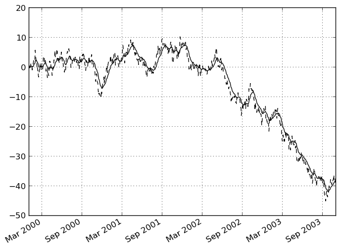
We can do a moving window regression to see how the relationship changes over time:

In [205]: model = ols(y=rets['AAPL'], x=rets.ix[:, ['GOOG']],
   .....:             window=250)
---------------------------------------------------------------------------
NameError                                 Traceback (most recent call last)
<ipython-input-205-77141e77cc71> in <module>()
----> 1 model = ols(y=rets['AAPL'], x=rets.ix[:, ['GOOG']],
      2              window=250)
NameError: name 'rets' is not defined

# just plot the coefficient for GOOG
In [206]: model.beta['GOOG'].plot()
---------------------------------------------------------------------------
NameError                                 Traceback (most recent call last)
<ipython-input-206-3fa2144a7140> in <module>()
----> 1 model.beta['GOOG'].plot()
NameError: name 'model' is not defined

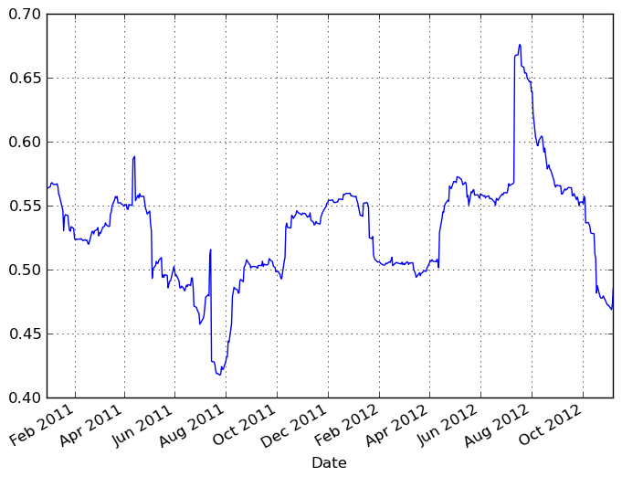
It looks like there are some outliers rolling in and out of the window in the above regression, influencing the results. We could perform a simple winsorization at the 3 STD level to trim the impact of outliers:

In [207]: winz = rets.copy()
---------------------------------------------------------------------------
NameError                                 Traceback (most recent call last)
<ipython-input-207-ef159cc28d64> in <module>()
----> 1 winz = rets.copy()
NameError: name 'rets' is not defined

In [208]: std_1year = rolling_std(rets, 250, min_periods=20)
---------------------------------------------------------------------------
NameError                                 Traceback (most recent call last)
<ipython-input-208-498f5e1a00b5> in <module>()
----> 1 std_1year = rolling_std(rets, 250, min_periods=20)
NameError: name 'rets' is not defined

# cap at 3 * 1 year standard deviation
In [209]: cap_level = 3 * np.sign(winz) * std_1year
---------------------------------------------------------------------------
NameError                                 Traceback (most recent call last)
<ipython-input-209-eceb7c33338e> in <module>()
----> 1 cap_level = 3 * np.sign(winz) * std_1year
NameError: name 'winz' is not defined

In [210]: winz[np.abs(winz) > 3 * std_1year] = cap_level
---------------------------------------------------------------------------
NameError                                 Traceback (most recent call last)
<ipython-input-210-dbfbe3507388> in <module>()
----> 1 winz[np.abs(winz) > 3 * std_1year] = cap_level
NameError: name 'cap_level' is not defined

In [211]: winz_model = ols(y=winz['AAPL'], x=winz.ix[:, ['GOOG']],
   .....:             window=250)
---------------------------------------------------------------------------
NameError                                 Traceback (most recent call last)
<ipython-input-211-71948d79df5f> in <module>()
----> 1 winz_model = ols(y=winz['AAPL'], x=winz.ix[:, ['GOOG']],
      2              window=250)
NameError: name 'winz' is not defined

In [212]: model.beta['GOOG'].plot(label="With outliers")
---------------------------------------------------------------------------
NameError                                 Traceback (most recent call last)
<ipython-input-212-bf6780a1eec6> in <module>()
----> 1 model.beta['GOOG'].plot(label="With outliers")
NameError: name 'model' is not defined

In [213]: winz_model.beta['GOOG'].plot(label="Winsorized"); plt.legend(loc='best')
---------------------------------------------------------------------------
NameError                                 Traceback (most recent call last)
<ipython-input-213-815cf4b32c25> in <module>()
----> 1 winz_model.beta['GOOG'].plot(label="Winsorized"); plt.legend(loc='best')
NameError: name 'winz_model' is not defined

So in this simple example we see the impact of winsorization is actually quite significant. Note the correlation after winsorization remains high:

In [214]: winz.corrwith(rets)
---------------------------------------------------------------------------
NameError                                 Traceback (most recent call last)
<ipython-input-214-0230c93d5cfd> in <module>()
----> 1 winz.corrwith(rets)
NameError: name 'winz' is not defined

Multiple regressions can be run by passing a DataFrame with multiple columns for the predictors x:

In [215]: ols(y=winz['AAPL'], x=winz.drop(['AAPL'], axis=1))
---------------------------------------------------------------------------
NameError                                 Traceback (most recent call last)
<ipython-input-215-de0445896065> in <module>()
----> 1 ols(y=winz['AAPL'], x=winz.drop(['AAPL'], axis=1))
NameError: name 'winz' is not defined

Panel regression¶

We’ve implemented moving window panel regression on potentially unbalanced panel data (see this article if this means nothing to you). Suppose we wanted to model the relationship between the magnitude of the daily return and trading volume among a group of stocks, and we want to pool all the data together to run one big regression. This is actually quite easy:

# make the units somewhat comparable
In [216]: volume = panel['Volume'] / 1e8
---------------------------------------------------------------------------
NameError                                 Traceback (most recent call last)
<ipython-input-216-81ef33fb51c8> in <module>()
----> 1 volume = panel['Volume'] / 1e8
NameError: name 'panel' is not defined

In [217]: model = ols(y=volume, x={'return' : np.abs(rets)})
---------------------------------------------------------------------------
NameError                                 Traceback (most recent call last)
<ipython-input-217-4e7bad5a4523> in <module>()
----> 1 model = ols(y=volume, x={'return' : np.abs(rets)})
NameError: name 'volume' is not defined

In [218]: model
---------------------------------------------------------------------------
NameError                                 Traceback (most recent call last)
<ipython-input-218-458d5f1afc81> in <module>()
----> 1 model
NameError: name 'model' is not defined

In a panel model, we can insert dummy (0-1) variables for the “entities” involved (here, each of the stocks) to account the a entity-specific effect (intercept):

In [219]: fe_model = ols(y=volume, x={'return' : np.abs(rets)},
   .....:                entity_effects=True)
---------------------------------------------------------------------------
NameError                                 Traceback (most recent call last)
<ipython-input-219-123d2b0e6684> in <module>()
----> 1 fe_model = ols(y=volume, x={'return' : np.abs(rets)},
      2                 entity_effects=True)
NameError: name 'volume' is not defined

In [220]: fe_model
---------------------------------------------------------------------------
NameError                                 Traceback (most recent call last)
<ipython-input-220-e0aa1859f068> in <module>()
----> 1 fe_model
NameError: name 'fe_model' is not defined

Because we ran the regression with an intercept, one of the dummy variables must be dropped or the design matrix will not be full rank. If we do not use an intercept, all of the dummy variables will be included:

In [221]: fe_model = ols(y=volume, x={'return' : np.abs(rets)},
   .....:                entity_effects=True, intercept=False)
---------------------------------------------------------------------------
NameError                                 Traceback (most recent call last)
<ipython-input-221-ebdd062db1f9> in <module>()
----> 1 fe_model = ols(y=volume, x={'return' : np.abs(rets)},
      2                 entity_effects=True, intercept=False)
NameError: name 'volume' is not defined

In [222]: fe_model
---------------------------------------------------------------------------
NameError                                 Traceback (most recent call last)
<ipython-input-222-e0aa1859f068> in <module>()
----> 1 fe_model
NameError: name 'fe_model' is not defined

We can also include time effects, which demeans the data cross-sectionally at each point in time (equivalent to including dummy variables for each date). More mathematical care must be taken to properly compute the standard errors in this case:

In [223]: te_model = ols(y=volume, x={'return' : np.abs(rets)},
   .....:                time_effects=True, entity_effects=True)
---------------------------------------------------------------------------
NameError                                 Traceback (most recent call last)
<ipython-input-223-c1e13ca06b73> in <module>()
----> 1 te_model = ols(y=volume, x={'return' : np.abs(rets)},
      2                 time_effects=True, entity_effects=True)
NameError: name 'volume' is not defined

In [224]: te_model
---------------------------------------------------------------------------
NameError                                 Traceback (most recent call last)
<ipython-input-224-b9166339d2b5> in <module>()
----> 1 te_model
NameError: name 'te_model' is not defined

Here the intercept (the mean term) is dropped by default because it will be 0 according to the model assumptions, having subtracted off the group means.

Result fields and tests¶

We’ll leave it to the user to explore the docstrings and source, especially as we’ll be moving this code into statsmodels in the near future.

pandas 0.7.3 documentation

Table Of Contents

Search

Computational tools¶

Statistical functions¶

Covariance¶

Correlation¶

Data ranking¶

Moving (rolling) statistics / moments¶

Binary rolling moments¶

Computing rolling pairwise correlations¶

Exponentially weighted moment functions¶

Linear and panel regression¶

Standard OLS regression¶

Panel regression¶

Result fields and tests¶