Group By: split-apply-combine
By “group by” we are refer to a process involving one or more of the following steps
- Splitting the data into groups based on some criteria
- Applying a function to each group independently
- Combining the results into a data structure
Of these, the split step is the most straightforward. In fact, in many situations you may wish to split the data set into groups and do something with those groups yourself. In the apply step, we might wish to one of the following:
Aggregation: computing a summary statistic (or statistics) about each group. Some examples:
- Compute group sums or means
- Compute group sizes / counts
Transformation: perform some group-specific computations and return a like-indexed. Some examples:
- Standardizing data (zscore) within group
- Filling NAs within groups with a value derived from each group
Some combination of the above: GroupBy will examine the results of the apply step and try to return a sensibly combined result if it doesn’t fit into either of the above two categories
Since the set of object instance method on pandas data structures are generally rich and expressive, we often simply want to invoke, say, a DataFrame function on each group. The name GroupBy should be quite familiar to those who have used a SQL-based tool (or itertools), in which you can write code like:
SELECT Column1, Column2, mean(Column3), sum(Column4)
FROM SomeTable
GROUP BY Column1, Column2
We aim to make operations like this natural and easy to express using pandas. We’ll address each area of GroupBy functionality then provide some non-trivial examples / use cases.
Splitting an object into groups
pandas objects can be split on any of their axes. The abstract definition of grouping is to provide a mapping of labels to group names. To create a GroupBy object (more on what the GroupBy object is later), you do the following:
>>> grouped = obj.groupby(key)
>>> grouped = obj.groupby(key, axis=1)
>>> grouped = obj.groupby([key1, key2])
The mapping can be specified many different ways:
- A Python function, to be called on each of the axis labels
- A list or NumPy array of the same length as the selected axis
- A dict or Series, providing a label -> group name mapping
- For DataFrame objects, a string indicating a column to be used to group. Of course df.groupby('A') is just syntactic sugar for df.groupby(df['A']), but it makes life simpler
- A list of any of the above things
Collectively we refer to the grouping objects as the keys. For example, consider the following DataFrame:
In [444]: df = DataFrame({'A' : ['foo', 'bar', 'foo', 'bar',
   .....:                        'foo', 'bar', 'foo', 'foo'],
   .....:                 'B' : ['one', 'one', 'two', 'three',
   .....:                        'two', 'two', 'one', 'three'],
   .....:                 'C' : randn(8), 'D' : randn(8)})
   .....:

In [445]: df
Out[445]:
     A      B         C         D
0  foo    one  0.469112 -0.861849
1  bar    one -0.282863 -2.104569
2  foo    two -1.509059 -0.494929
3  bar  three -1.135632  1.071804
4  foo    two  1.212112  0.721555
5  bar    two -0.173215 -0.706771
6  foo    one  0.119209 -1.039575
7  foo  three -1.044236  0.271860
We could naturally group by either the A or B columns or both:
In [446]: grouped = df.groupby('A')

In [447]: grouped = df.groupby(['A', 'B'])
These will split the DataFrame on its index (rows). We could also split by the columns:
In [448]: def get_letter_type(letter):
   .....:     if letter.lower() in 'aeiou':
   .....:         return 'vowel'
   .....:     else:
   .....:         return 'consonant'
   .....:

In [449]: grouped = df.groupby(get_letter_type, axis=1)
Starting with 0.8, pandas Index objects now supports duplicate values. If a non-unique index is used as the group key in a groupby operation, all values for the same index value will be considered to be in one group and thus the output of aggregation functions will only contain unique index values:
In [450]: lst = [1, 2, 3, 1, 2, 3]

In [451]: s = Series([1, 2, 3, 10, 20, 30], lst)

In [452]: grouped = s.groupby(level=0)

In [453]: grouped.first()
Out[453]:
1    1
2    2
3    3

In [454]: grouped.last()
Out[454]:
1    10
2    20
3    30

In [455]: grouped.sum()
Out[455]:
1    11
2    22
3    33
Note that no splitting occurs until it’s needed. Creating the GroupBy object only verifies that you’ve passed a valid mapping.
Note
Many kinds of complicated data manipulations can be expressed in terms of GroupBy operations (though can’t be guaranteed to be the most efficient). You can get quite creative with the label mapping functions.
GroupBy object attributes
The groups attribute is a dict whose keys are the computed unique groups and corresponding values being the axis labels belonging to each group. In the above example we have:
In [456]: df.groupby('A').groups
Out[456]: {'bar': [1, 3, 5], 'foo': [0, 2, 4, 6, 7]}

In [457]: df.groupby(get_letter_type, axis=1).groups
Out[457]: {'consonant': ['B', 'C', 'D'], 'vowel': ['A']}
Calling the standard Python len function on the GroupBy object just returns the length of the groups dict, so it is largely just a convenience:
In [458]: grouped = df.groupby(['A', 'B'])

In [459]: grouped.groups
Out[459]:
{('bar', 'one'): [1],
 ('bar', 'three'): [3],
 ('bar', 'two'): [5],
 ('foo', 'one'): [0, 6],
 ('foo', 'three'): [7],
 ('foo', 'two'): [2, 4]}

In [460]: len(grouped)
Out[460]: 6
By default the group keys are sorted during the groupby operation. You may however pass sort``=``False for potential speedups:
In [461]: df2 = DataFrame({'X' : ['B', 'B', 'A', 'A'], 'Y' : [1, 2, 3, 4]})

In [462]: df2.groupby(['X'], sort=True).sum()
Out[462]:
   Y
X
A  7
B  3

In [463]: df2.groupby(['X'], sort=False).sum()
Out[463]:
   Y
X
B  3
A  7
GroupBy with MultiIndex
With hierarchically-indexed data, it’s quite natural to group by one of the levels of the hierarchy.
In [464]: s
Out[464]:
first  second
bar    one      -0.424972
       two       0.567020
baz    one       0.276232
       two      -1.087401
foo    one      -0.673690
       two       0.113648
qux    one      -1.478427
       two       0.524988

In [465]: grouped = s.groupby(level=0)

In [466]: grouped.sum()
Out[466]:
first
bar      0.142048
baz     -0.811169
foo     -0.560041
qux     -0.953439
If the MultiIndex has names specified, these can be passed instead of the level number:
In [467]: s.groupby(level='second').sum()
Out[467]:
second
one      -2.300857
two       0.118256
The aggregation functions such as sum will take the level parameter directly. Additionally, the resulting index will be named according to the chosen level:
In [468]: s.sum(level='second')
Out[468]:
second
one      -2.300857
two       0.118256
Also as of v0.6, grouping with multiple levels is supported.
In [469]: s
Out[469]:
first  second  third
bar    doo     one      0.404705
               two      0.577046
baz    bee     one     -1.715002
               two     -1.039268
foo    bop     one     -0.370647
               two     -1.157892
qux    bop     one     -1.344312
               two      0.844885

In [470]: s.groupby(level=['first','second']).sum()
Out[470]:
first  second
bar    doo       0.981751
baz    bee      -2.754270
foo    bop      -1.528539
qux    bop      -0.499427
More on the sum function and aggregation later.
DataFrame column selection in GroupBy
Once you have created the GroupBy object from a DataFrame, for example, you might want to do something different for each of the columns. Thus, using [] similar to getting a column from a DataFrame, you can do:
In [471]: grouped = df.groupby(['A'])

In [472]: grouped_C = grouped['C']

In [473]: grouped_D = grouped['D']
This is mainly syntactic sugar for the alternative and much more verbose:
In [474]: df['C'].groupby(df['A'])
Out[474]: <pandas.core.groupby.SeriesGroupBy at 0x1166643d0>
Additionally this method avoids recomputing the internal grouping information derived from the passed key.
Iterating through groups
With the GroupBy object in hand, iterating through the grouped data is very natural and functions similarly to itertools.groupby:
In [475]: grouped = df.groupby('A')

In [476]: for name, group in grouped:
   .....:        print name
   .....:        print group
   .....:
bar
     A      B         C         D
1  bar    one -0.282863 -2.104569
3  bar  three -1.135632  1.071804
5  bar    two -0.173215 -0.706771
foo
     A      B         C         D
0  foo    one  0.469112 -0.861849
2  foo    two -1.509059 -0.494929
4  foo    two  1.212112  0.721555
6  foo    one  0.119209 -1.039575
7  foo  three -1.044236  0.271860
In the case of grouping by multiple keys, the group name will be a tuple:
In [477]: for name, group in df.groupby(['A', 'B']):
   .....:        print name
   .....:        print group
   .....:
('bar', 'one')
     A    B         C         D
1  bar  one -0.282863 -2.104569
('bar', 'three')
     A      B         C         D
3  bar  three -1.135632  1.071804
('bar', 'two')
     A    B         C         D
5  bar  two -0.173215 -0.706771
('foo', 'one')
     A    B         C         D
0  foo  one  0.469112 -0.861849
6  foo  one  0.119209 -1.039575
('foo', 'three')
     A      B         C        D
7  foo  three -1.044236  0.27186
('foo', 'two')
     A    B         C         D
2  foo  two -1.509059 -0.494929
4  foo  two  1.212112  0.721555
It’s standard Python-fu but remember you can unpack the tuple in the for loop statement if you wish: for (k1, k2), group in grouped:.
Aggregation
Once the GroupBy object has been created, several methods are available to perform a computation on the grouped data. An obvious one is aggregation via the aggregate or equivalently agg method:
In [478]: grouped = df.groupby('A')

In [479]: grouped.aggregate(np.sum)
Out[479]:
            C         D
A
bar -1.591710 -1.739537
foo -0.752861 -1.402938

In [480]: grouped = df.groupby(['A', 'B'])

In [481]: grouped.aggregate(np.sum)
Out[481]:
                  C         D
A   B
bar one   -0.282863 -2.104569
    three -1.135632  1.071804
    two   -0.173215 -0.706771
foo one    0.588321 -1.901424
    three -1.044236  0.271860
    two   -0.296946  0.226626
As you can see, the result of the aggregation will have the group names as the new index along the grouped axis. In the case of multiple keys, the result is a MultiIndex by default, though this can be changed by using the as_index option:
In [482]: grouped = df.groupby(['A', 'B'], as_index=False)

In [483]: grouped.aggregate(np.sum)
Out[483]:
     A      B         C         D
0  bar    one -0.282863 -2.104569
1  bar  three -1.135632  1.071804
2  bar    two -0.173215 -0.706771
3  foo    one  0.588321 -1.901424
4  foo  three -1.044236  0.271860
5  foo    two -0.296946  0.226626

In [484]: df.groupby('A', as_index=False).sum()
Out[484]:
     A         C         D
0  bar -1.591710 -1.739537
1  foo -0.752861 -1.402938
Note that you could use the reset_index DataFrame function to achieve the same result as the column names are stored in the resulting MultiIndex:
In [485]: df.groupby(['A', 'B']).sum().reset_index()
Out[485]:
     A      B         C         D
0  bar    one -0.282863 -2.104569
1  bar  three -1.135632  1.071804
2  bar    two -0.173215 -0.706771
3  foo    one  0.588321 -1.901424
4  foo  three -1.044236  0.271860
5  foo    two -0.296946  0.226626
Another simple aggregation example is to compute the size of each group. This is included in GroupBy as the size method. It returns a Series whose index are the group names and whose values are the sizes of each group.
In [486]: grouped.size()
Out[486]:
A    B
bar  one      1
     three    1
     two      1
foo  one      2
     three    1
     two      2
Applying multiple functions at once
With grouped Series you can also pass a list or dict of functions to do aggregation with, outputting a DataFrame:
In [487]: grouped = df.groupby('A')

In [488]: grouped['C'].agg([np.sum, np.mean, np.std])
Out[488]:
          sum      mean       std
A
bar -1.591710 -0.530570  0.526860
foo -0.752861 -0.150572  1.113308
If a dict is passed, the keys will be used to name the columns. Otherwise the function’s name (stored in the function object) will be used.
In [489]: grouped['D'].agg({'result1' : np.sum,
   .....:                   'result2' : np.mean})
   .....:
Out[489]:
      result2   result1
A
bar -0.579846 -1.739537
foo -0.280588 -1.402938
On a grouped DataFrame, you can pass a list of functions to apply to each column, which produces an aggregated result with a hierarchical index:
In [490]: grouped.agg([np.sum, np.mean, np.std])
Out[490]:
            C                             D
          sum      mean       std       sum      mean       std
A
bar -1.591710 -0.530570  0.526860 -1.739537 -0.579846  1.591986
foo -0.752861 -0.150572  1.113308 -1.402938 -0.280588  0.753219
Passing a dict of functions has different behavior by default, see the next section.
Applying different functions to DataFrame columns
By passing a dict to aggregate you can apply a different aggregation to the columns of a DataFrame:
In [491]: grouped.agg({'C' : np.sum,
   .....:              'D' : lambda x: np.std(x, ddof=1)})
   .....:
Out[491]:
            C         D
A
bar -1.591710  1.591986
foo -0.752861  0.753219
The function names can also be strings. In order for a string to be valid it must be either implemented on GroupBy or available via dispatching:
In [492]: grouped.agg({'C' : 'sum', 'D' : 'std'})
Out[492]:
            C         D
A
bar -1.591710  1.591986
foo -0.752861  0.753219
Cython-optimized aggregation functions
Some common aggregations, currently only sum, mean, and std, have optimized Cython implementations:
In [493]: df.groupby('A').sum()
Out[493]:
            C         D
A
bar -1.591710 -1.739537
foo -0.752861 -1.402938

In [494]: df.groupby(['A', 'B']).mean()
Out[494]:
                  C         D
A   B
bar one   -0.282863 -2.104569
    three -1.135632  1.071804
    two   -0.173215 -0.706771
foo one    0.294161 -0.950712
    three -1.044236  0.271860
    two   -0.148473  0.113313
Of course sum and mean are implemented on pandas objects, so the above code would work even without the special versions via dispatching (see below).
Transformation
The transform method returns an object that is indexed the same (same size) as the one being grouped. Thus, the passed transform function should return a result that is the same size as the group chunk. For example, suppose we wished to standardize the data within each group:
In [495]: index = date_range('10/1/1999', periods=1100)

In [496]: ts = Series(np.random.normal(0.5, 2, 1100), index)

In [497]: ts = rolling_mean(ts, 100, 100).dropna()

In [498]: ts.head()
Out[498]:
2000-01-08    0.536925
2000-01-09    0.494448
2000-01-10    0.496114
2000-01-11    0.443475
2000-01-12    0.474744
Freq: D

In [499]: ts.tail()
Out[499]:
2002-09-30    0.978859
2002-10-01    0.994704
2002-10-02    0.953789
2002-10-03    0.932345
2002-10-04    0.915581
Freq: D

In [500]: key = lambda x: x.year

In [501]: zscore = lambda x: (x - x.mean()) / x.std()

In [502]: transformed = ts.groupby(key).transform(zscore)
We would expect the result to now have mean 0 and standard deviation 1 within each group, which we can easily check:
# Original Data
In [503]: grouped = ts.groupby(key)

In [504]: grouped.mean()
Out[504]:
2000    0.416344
2001    0.416987
2002    0.599380

In [505]: grouped.std()
Out[505]:
2000    0.174755
2001    0.309640
2002    0.266172

# Transformed Data
In [506]: grouped_trans = transformed.groupby(key)

In [507]: grouped_trans.mean()
Out[507]:
2000   -0
2001   -0
2002   -0

In [508]: grouped_trans.std()
Out[508]:
2000    1
2001    1
2002    1
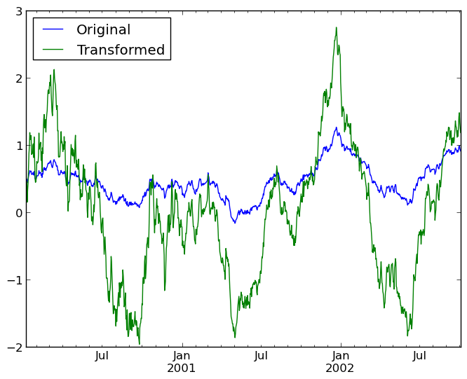
We can also visually compare the original and transformed data sets.
In [509]: compare = DataFrame({'Original': ts, 'Transformed': transformed})

In [510]: compare.plot()
Out[510]: <matplotlib.axes.AxesSubplot at 0x1139499d0>
Another common data transform is to replace missing data with the group mean.
In [511]: data_df
Out[511]:
<class 'pandas.core.frame.DataFrame'>
Int64Index: 1000 entries, 0 to 999
Data columns:
A    908  non-null values
B    953  non-null values
C    820  non-null values
dtypes: float64(3)

In [512]: countries = np.array(['US', 'UK', 'GR', 'JP'])

In [513]: key = countries[np.random.randint(0, 4, 1000)]

In [514]: grouped = data_df.groupby(key)

# Non-NA count in each group
In [515]: grouped.count()
Out[515]:
      A    B    C
GR  219  223  194
JP  238  250  211
UK  228  239  213
US  223  241  202

In [516]: f = lambda x: x.fillna(x.mean())

In [517]: transformed = grouped.transform(f)
We can verify that the group means have not changed in the transformed data and that the transformed data contains no NAs.
In [518]: grouped_trans = transformed.groupby(key)

In [519]: grouped.mean() # original group means
Out[519]:
           A         B         C
GR  0.093655 -0.004978 -0.049883
JP -0.067605  0.025828  0.006752
UK -0.054246  0.031742  0.068974
US  0.084334 -0.013433  0.056589

In [520]: grouped_trans.mean() # transformation did not change group means
Out[520]:
           A         B         C
GR  0.093655 -0.004978 -0.049883
JP -0.067605  0.025828  0.006752
UK -0.054246  0.031742  0.068974
US  0.084334 -0.013433  0.056589

In [521]: grouped.count() # original has some missing data points
Out[521]:
      A    B    C
GR  219  223  194
JP  238  250  211
UK  228  239  213
US  223  241  202

In [522]: grouped_trans.count() # counts after transformation
Out[522]:
      A    B    C
GR  234  234  234
JP  264  264  264
UK  251  251  251
US  251  251  251

In [523]: grouped_trans.size() # Verify non-NA count equals group size
Out[523]:
GR    234
JP    264
UK    251
US    251
Dispatching to instance methods
When doing an aggregation or transformation, you might just want to call an instance method on each data group. This is pretty easy to do by passing lambda functions:
In [524]: grouped = df.groupby('A')

In [525]: grouped.agg(lambda x: x.std())
Out[525]:
      B         C         D
A
bar NaN  0.526860  1.591986
foo NaN  1.113308  0.753219
But, it’s rather verbose and can be untidy if you need to pass additional arguments. Using a bit of metaprogramming cleverness, GroupBy now has the ability to “dispatch” method calls to the groups:
In [526]: grouped.std()
Out[526]:
            C         D
A
bar  0.526860  1.591986
foo  1.113308  0.753219
What is actually happening here is that a function wrapper is being generated. When invoked, it takes any passed arguments and invokes the function with any arguments on each group (in the above example, the std function). The results are then combined together much in the style of agg and transform (it actually uses apply to infer the gluing, documented next). This enables some operations to be carried out rather succinctly:
In [527]: tsdf = DataFrame(randn(1000, 3),
   .....:                  index=date_range('1/1/2000', periods=1000),
   .....:                  columns=['A', 'B', 'C'])
   .....:

In [528]: tsdf.ix[::2] = np.nan

In [529]: grouped = tsdf.groupby(lambda x: x.year)

In [530]: grouped.fillna(method='pad')
Out[530]:
<class 'pandas.core.frame.DataFrame'>
DatetimeIndex: 1000 entries, 2000-01-01 00:00:00 to 2002-09-26 00:00:00
Freq: D
Data columns:
A    998  non-null values
B    998  non-null values
C    998  non-null values
dtypes: float64(3)
In this example, we chopped the collection of time series into yearly chunks then independently called fillna on the groups.
Flexible apply
Some operations on the grouped data might not fit into either the aggregate or transform categories. Or, you may simply want GroupBy to infer how to combine the results. For these, use the apply function, which can be substituted for both aggregate and transform in many standard use cases. However, apply can handle some exceptional use cases, for example:
In [531]: df
Out[531]:
     A      B         C         D
0  foo    one  0.469112 -0.861849
1  bar    one -0.282863 -2.104569
2  foo    two -1.509059 -0.494929
3  bar  three -1.135632  1.071804
4  foo    two  1.212112  0.721555
5  bar    two -0.173215 -0.706771
6  foo    one  0.119209 -1.039575
7  foo  three -1.044236  0.271860

In [532]: grouped = df.groupby('A')

# could also just call .describe()
In [533]: grouped['C'].apply(lambda x: x.describe())
Out[533]:
A
bar  count    3.000000
     mean    -0.530570
     std      0.526860
     min     -1.135632
     25%     -0.709248
     50%     -0.282863
     75%     -0.228039
     max     -0.173215
foo  count    5.000000
     mean    -0.150572
     std      1.113308
     min     -1.509059
     25%     -1.044236
     50%      0.119209
     75%      0.469112
     max      1.212112
The dimension of the returned result can also change:
In [534]: grouped = df.groupby('A')['C']

In [535]: def f(group):
   .....:     return DataFrame({'original' : group,
   .....:                       'demeaned' : group - group.mean()})
   .....:

In [536]: grouped.apply(f)
Out[536]:
   demeaned  original
0  0.619685  0.469112
1  0.247707 -0.282863
2 -1.358486 -1.509059
3 -0.605062 -1.135632
4  1.362684  1.212112
5  0.357355 -0.173215
6  0.269781  0.119209
7 -0.893664 -1.044236
Other useful features
Automatic exclusion of “nuisance” columns
Again consider the example DataFrame we’ve been looking at:
In [537]: df
Out[537]:
     A      B         C         D
0  foo    one  0.469112 -0.861849
1  bar    one -0.282863 -2.104569
2  foo    two -1.509059 -0.494929
3  bar  three -1.135632  1.071804
4  foo    two  1.212112  0.721555
5  bar    two -0.173215 -0.706771
6  foo    one  0.119209 -1.039575
7  foo  three -1.044236  0.271860
Supposed we wished to compute the standard deviation grouped by the A column. There is a slight problem, namely that we don’t care about the data in column B. We refer to this as a “nuisance” column. If the passed aggregation function can’t be applied to some columns, the troublesome columns will be (silently) dropped. Thus, this does not pose any problems:
In [538]: df.groupby('A').std()
Out[538]:
            C         D
A
bar  0.526860  1.591986
foo  1.113308  0.753219
NA group handling
If there are any NaN values in the grouping key, these will be automatically excluded. So there will never be an “NA group”. This was not the case in older versions of pandas, but users were generally discarding the NA group anyway (and supporting it was an implementation headache).
Grouping with ordered factors
Categorical variables represented as instance of pandas’s Factor class can be used as group keys. If so, the order of the levels will be preserved:
In [539]: data = Series(np.random.randn(100))

In [540]: factor = qcut(data, [0, .25, .5, .75, 1.])

In [541]: data.groupby(factor).mean()
Out[541]:
[-3.713, -0.815]   -1.432664
(-0.815, 0.105]    -0.306693
(0.105, 0.609]      0.356789
(0.609, 2.154]      1.314491