

Intro to data structures#
We’ll start with a quick, non-comprehensive overview of the fundamental data structures in pandas to get you started. The fundamental behavior about data types, indexing, axis labeling, and alignment apply across all of the objects. To get started, import NumPy and load pandas into your namespace:
In [1]: import numpy as np

In [2]: import pandas as pd
Fundamentally, data alignment is intrinsic. The link between labels and data will not be broken unless done so explicitly by you.
We’ll give a brief intro to the data structures, then consider all of the broad categories of functionality and methods in separate sections.
Series#
Series is a one-dimensional labeled array capable of holding any data
type (integers, strings, floating point numbers, Python objects, etc.). The axis
labels are collectively referred to as the index. The basic method to create a Series is to call:
s = pd.Series(data, index=index)
Here, data can be many different things:
a Python dict
an ndarray
a scalar value (like 5)
The passed index is a list of axis labels. The constructor’s behavior depends on data’s type:
From ndarray
If data is an ndarray, index must be the same length as data. If no
index is passed, one will be created having values [0, ..., len(data) - 1].
In [3]: s = pd.Series(np.random.randn(5), index=["a", "b", "c", "d", "e"])

In [4]: s
Out[4]:
a    0.469112
b   -0.282863
c   -1.509059
d   -1.135632
e    1.212112
dtype: float64

In [5]: s.index
Out[5]: Index(['a', 'b', 'c', 'd', 'e'], dtype='str')

In [6]: pd.Series(np.random.randn(5))
Out[6]:
0   -0.173215
1    0.119209
2   -1.044236
3   -0.861849
4   -2.104569
dtype: float64
Note
pandas supports non-unique index values. If an operation that does not support duplicate index values is attempted, an exception will be raised at that time.
From dict
Series can be instantiated from dicts:
In [7]: d = {"b": 1, "a": 0, "c": 2}

In [8]: pd.Series(d)
Out[8]:
b    1
a    0
c    2
dtype: int64
If an index is passed, the values in data corresponding to the labels in the index will be pulled out.
In [9]: d = {"a": 0.0, "b": 1.0, "c": 2.0}

In [10]: pd.Series(d)
Out[10]:
a    0.0
b    1.0
c    2.0
dtype: float64

In [11]: pd.Series(d, index=["b", "c", "d", "a"])
Out[11]:
b    1.0
c    2.0
d    NaN
a    0.0
dtype: float64
Note
NaN (not a number) is the standard missing data marker used in pandas.
From scalar value
If data is a scalar value, the value will be repeated to match
the length of index. If the index is not provided, it defaults
to RangeIndex(1).
In [12]: pd.Series(5.0, index=["a", "b", "c", "d", "e"])
Out[12]:
a    5.0
b    5.0
c    5.0
d    5.0
e    5.0
dtype: float64
Series is ndarray-like#
Series acts very similarly to a numpy.ndarray and is a valid argument to most NumPy functions.
However, operations such as slicing will also slice the index.
In [13]: s.iloc[0]
Out[13]: np.float64(0.4691122999071863)

In [14]: s.iloc[:3]
Out[14]:
a    0.469112
b   -0.282863
c   -1.509059
dtype: float64

In [15]: s[s > s.median()]
Out[15]:
a    0.469112
e    1.212112
dtype: float64

In [16]: s.iloc[[4, 3, 1]]
Out[16]:
e    1.212112
d   -1.135632
b   -0.282863
dtype: float64

In [17]: np.exp(s)
Out[17]:
a    1.598575
b    0.753623
c    0.221118
d    0.321219
e    3.360575
dtype: float64
Note
We will address array-based indexing like s.iloc[[4, 3, 1]]
in the section on indexing.
Like a NumPy array, a pandas Series has a single dtype.
In [18]: s.dtype
Out[18]: dtype('float64')
This is often a NumPy dtype. However, pandas and 3rd-party libraries
extend NumPy’s type system in a few places, in which case the dtype would
be an ExtensionDtype. Some examples within
pandas are Categorical data and Nullable integer data type. See dtypes
for more.
If you need the actual array backing a Series, use Series.array.
In [19]: s.array
Out[19]:
<NumpyExtensionArray>
[ 0.4691122999071863, -0.2828633443286633, -1.5090585031735124,
 -1.1356323710171934,  1.2121120250208506]
Length: 5, dtype: float64
Accessing the array can be useful when you need to do some operation without the index (to disable automatic alignment, for example).
Series.array will always be an ExtensionArray.
Briefly, an ExtensionArray is a thin wrapper around one or more concrete arrays like a
numpy.ndarray. pandas knows how to take an ExtensionArray and
store it in a Series or a column of a DataFrame.
See dtypes for more.
While Series is ndarray-like, if you need an actual ndarray, then use
Series.to_numpy().
In [20]: s.to_numpy()
Out[20]: array([ 0.4691, -0.2829, -1.5091, -1.1356,  1.2121])
Even if the Series is backed by a ExtensionArray,
Series.to_numpy() will return a NumPy ndarray.
Series is dict-like#
A Series is also like a fixed-size dict in that you can get and set values by index
label:
In [21]: s["a"]
Out[21]: np.float64(0.4691122999071863)

In [22]: s["e"] = 12.0

In [23]: s
Out[23]:
a     0.469112
b    -0.282863
c    -1.509059
d    -1.135632
e    12.000000
dtype: float64

In [24]: "e" in s
Out[24]: True

In [25]: "f" in s
Out[25]: False
If a label is not contained in the index, an exception is raised:
In [26]: s["f"]
---------------------------------------------------------------------------
KeyError                                  Traceback (most recent call last)
File ~/work/pandas/pandas/pandas/core/indexes/base.py:3641, in Index.get_loc(self, key)
   3640 try:
-> 3641     return self._engine.get_loc(casted_key)
   3642 except KeyError as err:

File pandas/_libs/index.pyx:168, in pandas._libs.index.IndexEngine.get_loc()
--> 168 'Could not get source, probably due dynamically evaluated source code.'
File pandas/_libs/index.pyx:197, in pandas._libs.index.IndexEngine.get_loc()
--> 197 'Could not get source, probably due dynamically evaluated source code.'
File pandas/_libs/hashtable_class_helper.pxi:7668, in pandas._libs.hashtable.PyObjectHashTable.get_item()
-> 7668 'Could not get source, probably due dynamically evaluated source code.'
File pandas/_libs/hashtable_class_helper.pxi:7676, in pandas._libs.hashtable.PyObjectHashTable.get_item()
-> 7676 'Could not get source, probably due dynamically evaluated source code.'
KeyError: 'f'

The above exception was the direct cause of the following exception:

KeyError                                  Traceback (most recent call last)
Cell In[26], line 1
----> 1 s["f"]

File ~/work/pandas/pandas/pandas/core/series.py:959, in Series.__getitem__(self, key)
    954     key = unpack_1tuple(key)
    956 elif key_is_scalar:
    957     # Note: GH#50617 in 3.0 we changed int key to always be treated as
    958     #  a label, matching DataFrame behavior.
--> 959     return self._get_value(key)
    961 # Convert generator to list before going through hashable part
    962 # (We will iterate through the generator there to check for slices)
    963 if is_iterator(key):

File ~/work/pandas/pandas/pandas/core/series.py:1046, in Series._get_value(self, label, takeable)
   1043     return self._values[label]
   1045 # Similar to Index.get_value, but we do not fall back to positional
-> 1046 loc = self.index.get_loc(label)
   1048 if is_integer(loc):
   1049     return self._values[loc]

File ~/work/pandas/pandas/pandas/core/indexes/base.py:3648, in Index.get_loc(self, key)
   3643     if isinstance(casted_key, slice) or (
   3644         isinstance(casted_key, abc.Iterable)
   3645         and any(isinstance(x, slice) for x in casted_key)
   3646     ):
   3647         raise InvalidIndexError(key) from err
-> 3648     raise KeyError(key) from err
   3649 except TypeError:
   3650     # If we have a listlike key, _check_indexing_error will raise
   3651     #  InvalidIndexError. Otherwise we fall through and re-raise
   3652     #  the TypeError.
   3653     self._check_indexing_error(key)

KeyError: 'f'
Using the Series.get() method, a missing label will return None or specified default:
In [27]: s.get("f")

In [28]: s.get("f", np.nan)
Out[28]: nan
These labels can also be accessed by attribute.
Vectorized operations and label alignment with Series#
When working with raw NumPy arrays, looping through value-by-value is usually
not necessary. The same is true when working with Series in pandas.
Series can also be passed into most NumPy methods expecting an ndarray.
In [29]: s + s
Out[29]:
a     0.938225
b    -0.565727
c    -3.018117
d    -2.271265
e    24.000000
dtype: float64

In [30]: s * 2
Out[30]:
a     0.938225
b    -0.565727
c    -3.018117
d    -2.271265
e    24.000000
dtype: float64

In [31]: np.exp(s)
Out[31]:
a         1.598575
b         0.753623
c         0.221118
d         0.321219
e    162754.791419
dtype: float64
A key difference between Series and ndarray is that operations between Series
automatically align the data based on label. Thus, you can write computations
without giving consideration to whether the Series involved have the same
labels.
In [32]: s.iloc[1:] + s.iloc[:-1]
Out[32]:
a         NaN
b   -0.565727
c   -3.018117
d   -2.271265
e         NaN
dtype: float64
The result of an operation between unaligned Series will have the union of
the indexes involved. If a label is not found in one Series or the other, the
result will be marked as missing NaN. Being able to write code without doing
any explicit data alignment grants immense freedom and flexibility in
interactive data analysis and research. The integrated data alignment features
of the pandas data structures set pandas apart from the majority of related
tools for working with labeled data.
Note
In general, we chose to make the default result of operations between differently indexed objects yield the union of the indexes in order to avoid loss of information. Having an index label, though the data is missing, is typically important information as part of a computation. You of course have the option of dropping labels with missing data via the dropna function.
Name attribute#
Series also has a name attribute:
In [33]: s = pd.Series(np.random.randn(5), name="something")

In [34]: s
Out[34]:
0   -0.494929
1    1.071804
2    0.721555
3   -0.706771
4   -1.039575
Name: something, dtype: float64

In [35]: s.name
Out[35]: 'something'
The Series name can be assigned automatically in many cases, in particular,
when selecting a single column from a DataFrame, the name will be assigned
the column label.
You can rename a Series with the pandas.Series.rename() method.
In [36]: s2 = s.rename("different")

In [37]: s2.name
Out[37]: 'different'
Note that s and s2 refer to different objects.
DataFrame#
DataFrame is a 2-dimensional labeled data structure with columns of
potentially different types. You can think of it like a spreadsheet or SQL
table, or a dict of Series objects. It is generally the most commonly used
pandas object. Like Series, DataFrame accepts many different kinds of input:
Dict of 1D ndarrays, lists, dicts, or
Series2-D numpy.ndarray
Structured or record ndarray
A
SeriesAnother
DataFrame
Along with the data, you can optionally pass index (row labels) and columns (column labels) arguments. If you pass an index and / or columns, you are guaranteeing the index and / or columns of the resulting DataFrame. Thus, a dict of Series plus a specific index will discard all data not matching up to the passed index.
If axis labels are not passed, they will be constructed from the input data based on common sense rules.
From dict of Series or dicts#
The resulting index will be the union of the indexes of the various Series. If there are any nested dicts, these will first be converted to Series. If no columns are passed, the columns will be the ordered list of dict keys.
In [38]: d = {
   ....:     "one": pd.Series([1.0, 2.0, 3.0], index=["a", "b", "c"]),
   ....:     "two": pd.Series([1.0, 2.0, 3.0, 4.0], index=["a", "b", "c", "d"]),
   ....: }
   ....:

In [39]: df = pd.DataFrame(d)

In [40]: df
Out[40]:
   one  two
a  1.0  1.0
b  2.0  2.0
c  3.0  3.0
d  NaN  4.0

In [41]: pd.DataFrame(d, index=["d", "b", "a"])
Out[41]:
   one  two
d  NaN  4.0
b  2.0  2.0
a  1.0  1.0

In [42]: pd.DataFrame(d, index=["d", "b", "a"], columns=["two", "three"])
Out[42]:
   two three
d  4.0   NaN
b  2.0   NaN
a  1.0   NaN
The row and column labels can be accessed respectively by accessing the index and columns attributes:
Note
When a particular set of columns is passed along with a dict of data, the passed columns override the keys in the dict.
In [43]: df.index
Out[43]: Index(['a', 'b', 'c', 'd'], dtype='str')

In [44]: df.columns
Out[44]: Index(['one', 'two'], dtype='str')
From dict of ndarrays / lists#
All ndarrays must share the same length. If an index is passed, it must
also be the same length as the arrays. If no index is passed, the
result will be range(n), where n is the array length.
In [45]: d = {"one": [1.0, 2.0, 3.0, 4.0], "two": [4.0, 3.0, 2.0, 1.0]}

In [46]: pd.DataFrame(d)
Out[46]:
   one  two
0  1.0  4.0
1  2.0  3.0
2  3.0  2.0
3  4.0  1.0

In [47]: pd.DataFrame(d, index=["a", "b", "c", "d"])
Out[47]:
   one  two
a  1.0  4.0
b  2.0  3.0
c  3.0  2.0
d  4.0  1.0
From structured or record array#
This case is handled identically to a dict of arrays.
In [48]: data = np.zeros((2,), dtype=[("A", "i4"), ("B", "f4"), ("C", "S10")])

In [49]: data[:] = [(1, 2.0, "Hello"), (2, 3.0, "World")]

In [50]: pd.DataFrame(data)
Out[50]:
   A    B         C
0  1  2.0  b'Hello'
1  2  3.0  b'World'

In [51]: pd.DataFrame(data, index=["first", "second"])
Out[51]:
        A    B         C
first   1  2.0  b'Hello'
second  2  3.0  b'World'

In [52]: pd.DataFrame(data, columns=["C", "A", "B"])
Out[52]:
          C  A    B
0  b'Hello'  1  2.0
1  b'World'  2  3.0
Note
DataFrame is not intended to work exactly like a 2-dimensional NumPy ndarray.
From a list of dicts#
In [53]: data2 = [{"a": 1, "b": 2}, {"a": 5, "b": 10, "c": 20}]

In [54]: pd.DataFrame(data2)
Out[54]:
   a   b     c
0  1   2   NaN
1  5  10  20.0

In [55]: pd.DataFrame(data2, index=["first", "second"])
Out[55]:
        a   b     c
first   1   2   NaN
second  5  10  20.0

In [56]: pd.DataFrame(data2, columns=["a", "b"])
Out[56]:
   a   b
0  1   2
1  5  10
From a dict of tuples#
You can automatically create a MultiIndexed frame by passing a tuples dictionary.
In [57]: pd.DataFrame(
   ....:     {
   ....:         ("a", "b"): {("A", "B"): 1, ("A", "C"): 2},
   ....:         ("a", "a"): {("A", "C"): 3, ("A", "B"): 4},
   ....:         ("a", "c"): {("A", "B"): 5, ("A", "C"): 6},
   ....:         ("b", "a"): {("A", "C"): 7, ("A", "B"): 8},
   ....:         ("b", "b"): {("A", "D"): 9, ("A", "B"): 10},
   ....:     }
   ....: )
   ....:
Out[57]:
       a              b
       b    a    c    a     b
A B  1.0  4.0  5.0  8.0  10.0
  C  2.0  3.0  6.0  7.0   NaN
  D  NaN  NaN  NaN  NaN   9.0
From a Series#
The result will be a DataFrame with the same index as the input Series, and with one column whose name is the original name of the Series (only if no other column name provided).
In [58]: ser = pd.Series(range(3), index=list("abc"), name="ser")

In [59]: pd.DataFrame(ser)
Out[59]:
   ser
a    0
b    1
c    2
From a list of namedtuples#
The field names of the first namedtuple in the list determine the columns
of the DataFrame. The remaining namedtuples (or tuples) are simply unpacked
and their values are fed into the rows of the DataFrame. If any of those
tuples is shorter than the first namedtuple then the later columns in the
corresponding row are marked as missing values. If any are longer than the
first namedtuple, a ValueError is raised.
In [60]: from collections import namedtuple

In [61]: Point = namedtuple("Point", "x y")

In [62]: pd.DataFrame([Point(0, 0), Point(0, 3), (2, 3)])
Out[62]:
   x  y
0  0  0
1  0  3
2  2  3

In [63]: Point3D = namedtuple("Point3D", "x y z")

In [64]: pd.DataFrame([Point3D(0, 0, 0), Point3D(0, 3, 5), Point(2, 3)])
Out[64]:
   x  y    z
0  0  0  0.0
1  0  3  5.0
2  2  3  NaN
From a list of dataclasses#
Data Classes as introduced in PEP557, can be passed into the DataFrame constructor. Passing a list of dataclasses is equivalent to passing a list of dictionaries.
Please be aware, that all values in the list should be dataclasses, mixing
types in the list would result in a TypeError.
In [65]: from dataclasses import make_dataclass

In [66]: Point = make_dataclass("Point", [("x", int), ("y", int)])

In [67]: pd.DataFrame([Point(0, 0), Point(0, 3), Point(2, 3)])
Out[67]:
   x  y
0  0  0
1  0  3
2  2  3
Missing data
To construct a DataFrame with missing data, we use np.nan to
represent missing values. Alternatively, you may pass a numpy.MaskedArray
as the data argument to the DataFrame constructor, and its masked entries will
be considered missing. See Missing data for more.
Alternate constructors#
DataFrame.from_dict
DataFrame.from_dict() takes a dict of dicts or a dict of array-like sequences
and returns a DataFrame. It operates like the DataFrame constructor except
for the orient parameter which is 'columns' by default, but which can be
set to 'index' in order to use the dict keys as row labels.
In [68]: pd.DataFrame.from_dict(dict([("A", [1, 2, 3]), ("B", [4, 5, 6])]))
Out[68]:
   A  B
0  1  4
1  2  5
2  3  6
If you pass orient='index', the keys will be the row labels. In this
case, you can also pass the desired column names:
In [69]: pd.DataFrame.from_dict(
   ....:     dict([("A", [1, 2, 3]), ("B", [4, 5, 6])]),
   ....:     orient="index",
   ....:     columns=["one", "two", "three"],
   ....: )
   ....:
Out[69]:
   one  two  three
A    1    2      3
B    4    5      6
DataFrame.from_records
DataFrame.from_records() takes a list of tuples or an ndarray with structured
dtype. It works analogously to the normal DataFrame constructor, except that
the resulting DataFrame index may be a specific field of the structured
dtype.
In [70]: data
Out[70]:
array([(1, 2., b'Hello'), (2, 3., b'World')],
      dtype=[('A', '<i4'), ('B', '<f4'), ('C', 'S10')])

In [71]: pd.DataFrame.from_records(data, index="C")
Out[71]:
          A    B
C
b'Hello'  1  2.0
b'World'  2  3.0
Column selection, addition, deletion#
You can treat a DataFrame semantically like a dict of like-indexed Series
objects. Getting, setting, and deleting columns works with the same syntax as
the analogous dict operations:
In [72]: df["one"]
Out[72]:
a    1.0
b    2.0
c    3.0
d    NaN
Name: one, dtype: float64

In [73]: df["three"] = df["one"] * df["two"]

In [74]: df["flag"] = df["one"] > 2

In [75]: df
Out[75]:
   one  two  three   flag
a  1.0  1.0    1.0  False
b  2.0  2.0    4.0  False
c  3.0  3.0    9.0   True
d  NaN  4.0    NaN  False
Columns can be deleted or popped like with a dict:
In [76]: del df["two"]

In [77]: three = df.pop("three")

In [78]: df
Out[78]:
   one   flag
a  1.0  False
b  2.0  False
c  3.0   True
d  NaN  False
When inserting a scalar value, it will naturally be propagated to fill the column:
In [79]: df["foo"] = "bar"

In [80]: df
Out[80]:
   one   flag  foo
a  1.0  False  bar
b  2.0  False  bar
c  3.0   True  bar
d  NaN  False  bar
When inserting a Series that does not have the same index as the DataFrame, it
will be conformed to the DataFrame’s index:
In [81]: df["one_trunc"] = df["one"][:2]

In [82]: df
Out[82]:
   one   flag  foo  one_trunc
a  1.0  False  bar        1.0
b  2.0  False  bar        2.0
c  3.0   True  bar        NaN
d  NaN  False  bar        NaN
You can insert raw ndarrays but their length must match the length of the DataFrame’s index.
By default, columns get inserted at the end. DataFrame.insert()
inserts at a particular location in the columns:
In [83]: df.insert(1, "bar", df["one"])

In [84]: df
Out[84]:
   one  bar   flag  foo  one_trunc
a  1.0  1.0  False  bar        1.0
b  2.0  2.0  False  bar        2.0
c  3.0  3.0   True  bar        NaN
d  NaN  NaN  False  bar        NaN
Assigning new columns in method chains#
Inspired by dplyr’s
mutate verb, DataFrame has an assign()
method that allows you to easily create new columns that are potentially
derived from existing columns.
In [85]: iris = pd.read_csv("data/iris.data")

In [86]: iris.head()
Out[86]:
   SepalLength  SepalWidth  PetalLength  PetalWidth         Name
0          5.1         3.5          1.4         0.2  Iris-setosa
1          4.9         3.0          1.4         0.2  Iris-setosa
2          4.7         3.2          1.3         0.2  Iris-setosa
3          4.6         3.1          1.5         0.2  Iris-setosa
4          5.0         3.6          1.4         0.2  Iris-setosa

In [87]: iris.assign(sepal_ratio=iris["SepalWidth"] / iris["SepalLength"]).head()
Out[87]:
   SepalLength  SepalWidth  PetalLength  PetalWidth         Name  sepal_ratio
0          5.1         3.5          1.4         0.2  Iris-setosa     0.686275
1          4.9         3.0          1.4         0.2  Iris-setosa     0.612245
2          4.7         3.2          1.3         0.2  Iris-setosa     0.680851
3          4.6         3.1          1.5         0.2  Iris-setosa     0.673913
4          5.0         3.6          1.4         0.2  Iris-setosa     0.720000
In the example above, we inserted a precomputed value. We can also pass in a function of one argument to be evaluated on the DataFrame being assigned to.
In [88]: iris.assign(sepal_ratio=lambda x: (x["SepalWidth"] / x["SepalLength"])).head()
Out[88]:
   SepalLength  SepalWidth  PetalLength  PetalWidth         Name  sepal_ratio
0          5.1         3.5          1.4         0.2  Iris-setosa     0.686275
1          4.9         3.0          1.4         0.2  Iris-setosa     0.612245
2          4.7         3.2          1.3         0.2  Iris-setosa     0.680851
3          4.6         3.1          1.5         0.2  Iris-setosa     0.673913
4          5.0         3.6          1.4         0.2  Iris-setosa     0.720000
or, using pandas.col():
In [89]: iris.assign(sepal_ratio=pd.col("SepalWidth") / pd.col("SepalLength")).head()
Out[89]:
   SepalLength  SepalWidth  PetalLength  PetalWidth         Name  sepal_ratio
0          5.1         3.5          1.4         0.2  Iris-setosa     0.686275
1          4.9         3.0          1.4         0.2  Iris-setosa     0.612245
2          4.7         3.2          1.3         0.2  Iris-setosa     0.680851
3          4.6         3.1          1.5         0.2  Iris-setosa     0.673913
4          5.0         3.6          1.4         0.2  Iris-setosa     0.720000
assign() always returns a copy of the data, leaving the original
DataFrame untouched.
Passing a callable, as opposed to an actual value to be inserted, is
useful when you don’t have a reference to the DataFrame at hand. This is
common when using assign() in a chain of operations. For example,
we can limit the DataFrame to just those observations with a Sepal Length
greater than 5, calculate the ratio, and plot:
In [90]: (
   ....:     iris.query("SepalLength > 5")
   ....:     .assign(
   ....:         SepalRatio=lambda x: x.SepalWidth / x.SepalLength,
   ....:         PetalRatio=lambda x: x.PetalWidth / x.PetalLength,
   ....:     )
   ....:     .plot(kind="scatter", x="SepalRatio", y="PetalRatio")
   ....: )
   ....:
Out[90]: <Axes: xlabel='SepalRatio', ylabel='PetalRatio'>
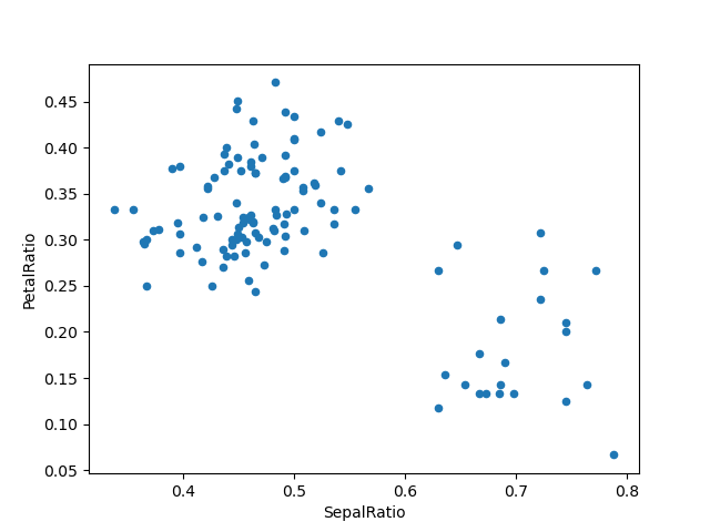
Since a function is passed in, the function is computed on the DataFrame being assigned to. Importantly, this is the DataFrame that’s been filtered to those rows with sepal length greater than 5. The filtering happens first, and then the ratio calculations. This is an example where we didn’t have a reference to the filtered DataFrame available.
The function signature for assign() is simply **kwargs. The keys
are the column names for the new fields, and the values are either a value
to be inserted (for example, a Series or NumPy array), or a function
of one argument to be called on the DataFrame. A copy of the original
DataFrame is returned, with the new values inserted.
The order of **kwargs is preserved. This allows
for dependent assignment, where an expression later in **kwargs can refer
to a column created earlier in the same assign().
In [91]: dfa = pd.DataFrame({"A": [1, 2, 3], "B": [4, 5, 6]})

In [92]: dfa.assign(C=lambda x: x["A"] + x["B"], D=lambda x: x["A"] + x["C"])
Out[92]:
   A  B  C   D
0  1  4  5   6
1  2  5  7   9
2  3  6  9  12
In the second expression, x['C'] will refer to the newly created column,
that’s equal to dfa['A'] + dfa['B'].
Indexing / selection#
The basics of indexing are as follows:
Operation |
Syntax |
Result |
|---|---|---|
Select column |
|
Series |
Select row by label |
|
Series |
Select row by integer location |
|
Series |
Slice rows |
|
DataFrame |
Select rows by boolean vector |
|
DataFrame |
Row selection, for example, returns a Series whose index is the columns of the
DataFrame:
In [93]: df.loc["b"]
Out[93]:
one            2.0
bar            2.0
flag         False
foo            bar
one_trunc      2.0
Name: b, dtype: object

In [94]: df.iloc[2]
Out[94]:
one           3.0
bar           3.0
flag         True
foo           bar
one_trunc     NaN
Name: c, dtype: object
For a more exhaustive treatment of sophisticated label-based indexing and slicing, see the section on indexing. We will address the fundamentals of reindexing / conforming to new sets of labels in the section on reindexing.
Data alignment and arithmetic#
Data alignment between DataFrame objects automatically align on both the
columns and the index (row labels). Again, the resulting object will have the
union of the column and row labels.
In [95]: df = pd.DataFrame(np.random.randn(10, 4), columns=["A", "B", "C", "D"])

In [96]: df2 = pd.DataFrame(np.random.randn(7, 3), columns=["A", "B", "C"])

In [97]: df + df2
Out[97]:
          A         B         C   D
0  0.045691 -0.014138  1.380871 NaN
1 -0.955398 -1.501007  0.037181 NaN
2 -0.662690  1.534833 -0.859691 NaN
3 -2.452949  1.237274 -0.133712 NaN
4  1.414490  1.951676 -2.320422 NaN
5 -0.494922 -1.649727 -1.084601 NaN
6 -1.047551 -0.748572 -0.805479 NaN
7       NaN       NaN       NaN NaN
8       NaN       NaN       NaN NaN
9       NaN       NaN       NaN NaN
When doing an operation between DataFrame and Series, the default behavior is
to align the Series index on the DataFrame columns, thus broadcasting
row-wise. For example:
In [98]: df - df.iloc[0]
Out[98]:
          A         B         C         D
0  0.000000  0.000000  0.000000  0.000000
1 -1.359261 -0.248717 -0.453372 -1.754659
2  0.253128  0.829678  0.010026 -1.991234
3 -1.311128  0.054325 -1.724913 -1.620544
4  0.573025  1.500742 -0.676070  1.367331
5 -1.741248  0.781993 -1.241620 -2.053136
6 -1.240774 -0.869551 -0.153282  0.000430
7 -0.743894  0.411013 -0.929563 -0.282386
8 -1.194921  1.320690  0.238224 -1.482644
9  2.293786  1.856228  0.773289 -1.446531
For explicit control over the matching and broadcasting behavior, see the section on flexible binary operations.
Arithmetic operations with scalars operate element-wise:
In [99]: df * 5 + 2
Out[99]:
           A         B         C          D
0   3.359299 -0.124862  4.835102   3.381160
1  -3.437003 -1.368449  2.568242  -5.392133
2   4.624938  4.023526  4.885230  -6.575010
3  -3.196342  0.146766 -3.789461  -4.721559
4   6.224426  7.378849  1.454750  10.217815
5  -5.346940  3.785103 -1.373001  -6.884519
6  -2.844569 -4.472618  4.068691   3.383309
7  -0.360173  1.930201  0.187285   1.969232
8  -2.615303  6.478587  6.026220  -4.032059
9  14.828230  9.156280  8.701544  -3.851494

In [100]: 1 / df
Out[100]:
          A          B         C           D
0  3.678365  -2.353094  1.763605    3.620145
1 -0.919624  -1.484363  8.799067   -0.676395
2  1.904807   2.470934  1.732964   -0.583090
3 -0.962215  -2.697986 -0.863638   -0.743875
4  1.183593   0.929567 -9.170108    0.608434
5 -0.680555   2.800959 -1.482360   -0.562777
6 -1.032084  -0.772485  2.416988    3.614523
7 -2.118489 -71.634509 -2.758294 -162.507295
8 -1.083352   1.116424  1.241860   -0.828904
9  0.389765   0.698687  0.746097   -0.854483

In [101]: df ** 4
Out[101]:
           A             B         C             D
0   0.005462  3.261689e-02  0.103370  5.822320e-03
1   1.398165  2.059869e-01  0.000167  4.777482e+00
2   0.075962  2.682596e-02  0.110877  8.650845e+00
3   1.166571  1.887302e-02  1.797515  3.265879e+00
4   0.509555  1.339298e+00  0.000141  7.297019e+00
5   4.661717  1.624699e-02  0.207103  9.969092e+00
6   0.881334  2.808277e+00  0.029302  5.858632e-03
7   0.049647  3.797614e-08  0.017276  1.433866e-09
8   0.725974  6.437005e-01  0.420446  2.118275e+00
9  43.329821  4.196326e+00  3.227153  1.875802e+00
Boolean operators operate element-wise as well:
In [102]: df1 = pd.DataFrame({"a": [1, 0, 1], "b": [0, 1, 1]}, dtype=bool)

In [103]: df2 = pd.DataFrame({"a": [0, 1, 1], "b": [1, 1, 0]}, dtype=bool)

In [104]: df1 & df2
Out[104]:
       a      b
0  False  False
1  False   True
2   True  False

In [105]: df1 | df2
Out[105]:
      a     b
0  True  True
1  True  True
2  True  True

In [106]: df1 ^ df2
Out[106]:
       a      b
0   True   True
1   True  False
2  False   True

In [107]: -df1
Out[107]:
       a      b
0  False   True
1   True  False
2  False  False
Transposing#
To transpose, access the T attribute or DataFrame.transpose(),
similar to an ndarray:
# only show the first 5 rows
In [108]: df[:5].T
Out[108]:
          0         1         2         3         4
A  0.271860 -1.087401  0.524988 -1.039268  0.844885
B -0.424972 -0.673690  0.404705 -0.370647  1.075770
C  0.567020  0.113648  0.577046 -1.157892 -0.109050
D  0.276232 -1.478427 -1.715002 -1.344312  1.643563
DataFrame interoperability with NumPy functions#
Most NumPy functions can be called directly on Series and DataFrame.
In [109]: np.exp(df)
Out[109]:
           A         B         C         D
0   1.312403  0.653788  1.763006  1.318154
1   0.337092  0.509824  1.120358  0.227996
2   1.690438  1.498861  1.780770  0.179963
3   0.353713  0.690288  0.314148  0.260719
4   2.327710  2.932249  0.896686  5.173571
5   0.230066  1.429065  0.509360  0.169161
6   0.379495  0.274028  1.512461  1.318720
7   0.623732  0.986137  0.695904  0.993865
8   0.397301  2.449092  2.237242  0.299269
9  13.009059  4.183951  3.820223  0.310274

In [110]: np.asarray(df)
Out[110]:
array([[ 0.2719, -0.425 ,  0.567 ,  0.2762],
       [-1.0874, -0.6737,  0.1136, -1.4784],
       [ 0.525 ,  0.4047,  0.577 , -1.715 ],
       [-1.0393, -0.3706, -1.1579, -1.3443],
       [ 0.8449,  1.0758, -0.109 ,  1.6436],
       [-1.4694,  0.357 , -0.6746, -1.7769],
       [-0.9689, -1.2945,  0.4137,  0.2767],
       [-0.472 , -0.014 , -0.3625, -0.0062],
       [-0.9231,  0.8957,  0.8052, -1.2064],
       [ 2.5656,  1.4313,  1.3403, -1.1703]])
DataFrame is not intended to be a drop-in replacement for ndarray as its
indexing semantics and data model are quite different in places from an n-dimensional
array.
Series implements __array_ufunc__, which allows it to work with NumPy’s
universal functions.
The ufunc is applied to the underlying array in a Series.
In [111]: ser = pd.Series([1, 2, 3, 4])

In [112]: np.exp(ser)
Out[112]:
0     2.718282
1     7.389056
2    20.085537
3    54.598150
dtype: float64
When multiple Series are passed to a ufunc, they are aligned before
performing the operation.
Like other parts of the library, pandas will automatically align labeled inputs
as part of a ufunc with multiple inputs. For example, using numpy.remainder()
on two Series with differently ordered labels will align before the operation.
In [113]: ser1 = pd.Series([1, 2, 3], index=["a", "b", "c"])

In [114]: ser2 = pd.Series([1, 3, 5], index=["b", "a", "c"])

In [115]: ser1
Out[115]:
a    1
b    2
c    3
dtype: int64

In [116]: ser2
Out[116]:
b    1
a    3
c    5
dtype: int64

In [117]: np.remainder(ser1, ser2)
Out[117]:
a    1
b    0
c    3
dtype: int64
As usual, the union of the two indices is taken, and non-overlapping values are filled with missing values.
In [118]: ser3 = pd.Series([2, 4, 6], index=["b", "c", "d"])

In [119]: ser3
Out[119]:
b    2
c    4
d    6
dtype: int64

In [120]: np.remainder(ser1, ser3)
Out[120]:
a    NaN
b    0.0
c    3.0
d    NaN
dtype: float64
When a binary ufunc is applied to a Series and Index, the Series
implementation takes precedence and a Series is returned.
In [121]: ser = pd.Series([1, 2, 3])

In [122]: idx = pd.Index([4, 5, 6])

In [123]: np.maximum(ser, idx)
Out[123]:
0    4
1    5
2    6
dtype: int64
NumPy ufuncs are safe to apply to Series backed by non-ndarray arrays,
for example arrays.SparseArray (see Sparse calculation). If possible,
the ufunc is applied without converting the underlying data to an ndarray.
Console display#
A very large DataFrame will be truncated to display them in the console.
You can also get a summary using info().
(The baseball dataset is from the plyr R package):
In [124]: baseball = pd.read_csv("data/baseball.csv")

In [125]: print(baseball)
       id     player  year  stint team  lg  ...    so  ibb  hbp   sh   sf  gidp
0   88641  womacto01  2006      2  CHN  NL  ...   4.0  0.0  0.0  3.0  0.0   0.0
1   88643  schilcu01  2006      1  BOS  AL  ...   1.0  0.0  0.0  0.0  0.0   0.0
..    ...        ...   ...    ...  ...  ..  ...   ...  ...  ...  ...  ...   ...
98  89533   aloumo01  2007      1  NYN  NL  ...  30.0  5.0  2.0  0.0  3.0  13.0
99  89534  alomasa02  2007      1  NYN  NL  ...   3.0  0.0  0.0  0.0  0.0   0.0

[100 rows x 23 columns]

In [126]: baseball.info()
<class 'pandas.DataFrame'>
RangeIndex: 100 entries, 0 to 99
Data columns (total 23 columns):
 #   Column  Non-Null Count  Dtype
---  ------  --------------  -----
 0   id      100 non-null    int64
 1   player  100 non-null    str
 2   year    100 non-null    int64
 3   stint   100 non-null    int64
 4   team    100 non-null    str
 5   lg      100 non-null    str
 6   g       100 non-null    int64
 7   ab      100 non-null    int64
 8   r       100 non-null    int64
 9   h       100 non-null    int64
 10  X2b     100 non-null    int64
 11  X3b     100 non-null    int64
 12  hr      100 non-null    int64
 13  rbi     100 non-null    float64
 14  sb      100 non-null    float64
 15  cs      100 non-null    float64
 16  bb      100 non-null    int64
 17  so      100 non-null    float64
 18  ibb     100 non-null    float64
 19  hbp     100 non-null    float64
 20  sh      100 non-null    float64
 21  sf      100 non-null    float64
 22  gidp    100 non-null    float64
dtypes: float64(9), int64(11), str(3)
memory usage: 19.5 KB
However, using DataFrame.to_string() will return a string representation of the
DataFrame in tabular form, though it won’t always fit the console width:
In [127]: print(baseball.iloc[-20:, :12].to_string())
       id     player  year  stint team  lg    g   ab   r    h  X2b  X3b
80  89474  finlest01  2007      1  COL  NL   43   94   9   17    3    0
81  89480  embreal01  2007      1  OAK  AL    4    0   0    0    0    0
82  89481  edmonji01  2007      1  SLN  NL  117  365  39   92   15    2
83  89482  easleda01  2007      1  NYN  NL   76  193  24   54    6    0
84  89489  delgaca01  2007      1  NYN  NL  139  538  71  139   30    0
85  89493  cormirh01  2007      1  CIN  NL    6    0   0    0    0    0
86  89494  coninje01  2007      2  NYN  NL   21   41   2    8    2    0
87  89495  coninje01  2007      1  CIN  NL   80  215  23   57   11    1
88  89497  clemero02  2007      1  NYA  AL    2    2   0    1    0    0
89  89498  claytro01  2007      2  BOS  AL    8    6   1    0    0    0
90  89499  claytro01  2007      1  TOR  AL   69  189  23   48   14    0
91  89501  cirilje01  2007      2  ARI  NL   28   40   6    8    4    0
92  89502  cirilje01  2007      1  MIN  AL   50  153  18   40    9    2
93  89521  bondsba01  2007      1  SFN  NL  126  340  75   94   14    0
94  89523  biggicr01  2007      1  HOU  NL  141  517  68  130   31    3
95  89525  benitar01  2007      2  FLO  NL   34    0   0    0    0    0
96  89526  benitar01  2007      1  SFN  NL   19    0   0    0    0    0
97  89530  ausmubr01  2007      1  HOU  NL  117  349  38   82   16    3
98  89533   aloumo01  2007      1  NYN  NL   87  328  51  112   19    1
99  89534  alomasa02  2007      1  NYN  NL    8   22   1    3    1    0
Wide DataFrames will be printed across multiple rows by default:
In [128]: pd.DataFrame(np.random.randn(3, 12))
Out[128]:
         0         1         2   ...        9         10        11
0 -1.226825  0.769804 -1.281247  ... -1.110336 -0.619976  0.149748
1 -0.732339  0.687738  0.176444  ...  1.462696 -1.743161 -0.826591
2 -0.345352  1.314232  0.690579  ...  0.896171 -0.487602 -0.082240

[3 rows x 12 columns]
You can change how much to print on a single row by setting the display.width
option:
In [129]: pd.set_option("display.width", 40)  # default is 80

In [130]: pd.DataFrame(np.random.randn(3, 12))
Out[130]:
         0         1         2   ...        9         10        11
0 -2.182937  0.380396  0.084844  ... -0.023688  2.410179  1.450520
1  0.206053 -0.251905 -2.213588  ... -0.025747 -0.988387  0.094055
2  1.262731  1.289997  0.082423  ... -0.281461  0.030711  0.109121

[3 rows x 12 columns]
You can adjust the max width of the individual columns by setting display.max_colwidth
In [131]: datafile = {
   .....:     "filename": ["filename_01", "filename_02"],
   .....:     "path": [
   .....:         "media/user_name/storage/folder_01/filename_01",
   .....:         "media/user_name/storage/folder_02/filename_02",
   .....:     ],
   .....: }
   .....:

In [132]: pd.set_option("display.max_colwidth", 30)

In [133]: pd.DataFrame(datafile)
Out[133]:
      filename                           path
0  filename_01  media/user_name/storage/fo...
1  filename_02  media/user_name/storage/fo...

In [134]: pd.set_option("display.max_colwidth", 100)

In [135]: pd.DataFrame(datafile)
Out[135]:
      filename                                           path
0  filename_01  media/user_name/storage/folder_01/filename_01
1  filename_02  media/user_name/storage/folder_02/filename_02
You can also disable this feature via the expand_frame_repr option.
This will print the table in one block.
DataFrame column attribute access and IPython completion#
If a DataFrame column label is a valid Python variable name, the column can be
accessed like an attribute:
In [136]: df = pd.DataFrame({"foo1": np.random.randn(5), "foo2": np.random.randn(5)})

In [137]: df
Out[137]:
       foo1      foo2
0  1.126203  0.781836
1 -0.977349 -1.071357
2  1.474071  0.441153
3 -0.064034  2.353925
4 -1.282782  0.583787

In [138]: df.foo1
Out[138]:
0    1.126203
1   -0.977349
2    1.474071
3   -0.064034
4   -1.282782
Name: foo1, dtype: float64
The columns are also connected to the IPython completion mechanism so they can be tab-completed:
In [5]: df.foo<TAB>  # noqa: E225, E999
df.foo1  df.foo2