

Chart visualization#
Note
The examples below assume that you’re using Jupyter.
This section demonstrates visualization through charting. For information on visualization of tabular data please see the section on Table Visualization.
We use the standard convention for referencing the matplotlib API:
In [1]: import matplotlib.pyplot as plt

In [2]: plt.close("all")
We provide the basics in pandas to easily create decent looking plots. See the ecosystem page for visualization libraries that go beyond the basics documented here.
Note
All calls to np.random are seeded with 123456.
Basic plotting: plot#
We will demonstrate the basics, see the cookbook for some advanced strategies.
The plot method on Series and DataFrame is just a simple wrapper around
plt.plot():
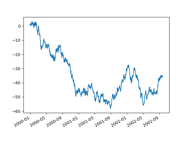
In [3]: np.random.seed(123456)

In [4]: ts = pd.Series(np.random.randn(1000), index=pd.date_range("1/1/2000", periods=1000))

In [5]: ts = ts.cumsum()

In [6]: ts.plot();
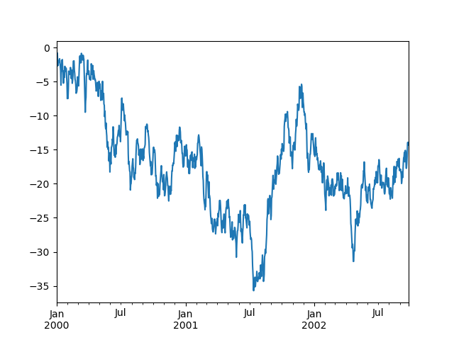
If the index consists of dates, it calls gcf().autofmt_xdate()
to try to format the x-axis nicely as per above.
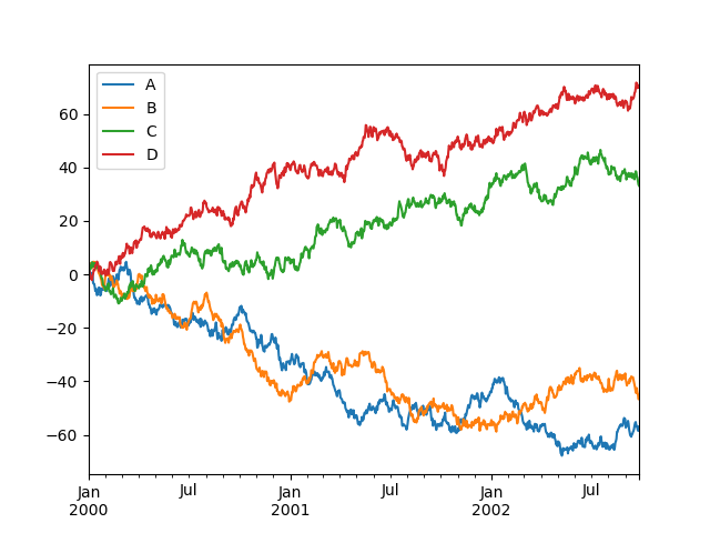
On DataFrame, plot() is a convenience to plot all of the columns with labels:
In [7]: df = pd.DataFrame(np.random.randn(1000, 4), index=ts.index, columns=list("ABCD"))

In [8]: df = df.cumsum()

In [9]: plt.figure();

In [10]: df.plot();
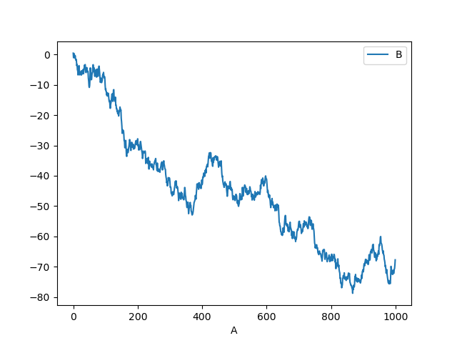
You can plot one column versus another using the x and y keywords in
plot():
In [11]: df3 = pd.DataFrame(np.random.randn(1000, 2), columns=["B", "C"]).cumsum()

In [12]: df3["A"] = pd.Series(list(range(len(df))))

In [13]: df3.plot(x="A", y="B");
Note
For more formatting and styling options, see formatting below.
Other plots#
Plotting methods allow for a handful of plot styles other than the
default line plot. These methods can be provided as the kind
keyword argument to plot(), and include:
‘hist’ for histogram
‘box’ for boxplot
‘area’ for area plots
‘scatter’ for scatter plots
‘hexbin’ for hexagonal bin plots
‘pie’ for pie plots
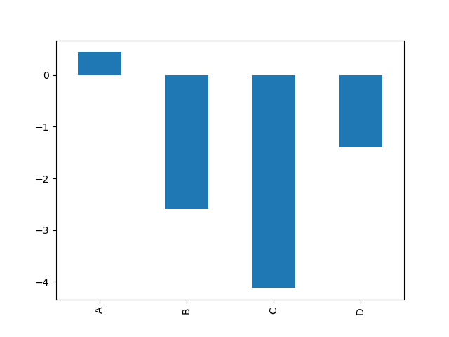
For example, a bar plot can be created the following way:
In [14]: plt.figure();

In [15]: df.iloc[5].plot(kind="bar");
You can also create these other plots using the methods DataFrame.plot.<kind> instead of providing the kind keyword argument. This makes it easier to discover plot methods and the specific arguments they use:
In [16]: df = pd.DataFrame()

In [17]: df.plot.<TAB>  # noqa: E225, E999
df.plot.area     df.plot.barh     df.plot.density  df.plot.hist     df.plot.line     df.plot.scatter
df.plot.bar      df.plot.box      df.plot.hexbin   df.plot.kde      df.plot.pie
In addition to these kind s, there are the DataFrame.hist(),
and DataFrame.boxplot() methods, which use a separate interface.
Finally, there are several plotting functions in pandas.plotting
that take a Series or DataFrame as an argument. These
include:
Plots may also be adorned with errorbars or tables.
Bar plots#
For labeled, non-time series data, you may wish to produce a bar plot:
In [18]: plt.figure();

In [19]: df.iloc[5].plot.bar();

In [20]: plt.axhline(0, color="k");
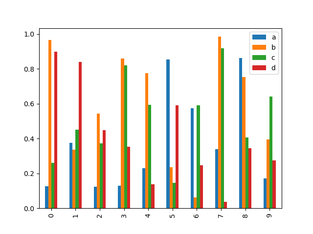
Calling a DataFrame’s plot.bar() method produces a multiple
bar plot:
In [21]: df2 = pd.DataFrame(np.random.rand(10, 4), columns=["a", "b", "c", "d"])

In [22]: df2.plot.bar();
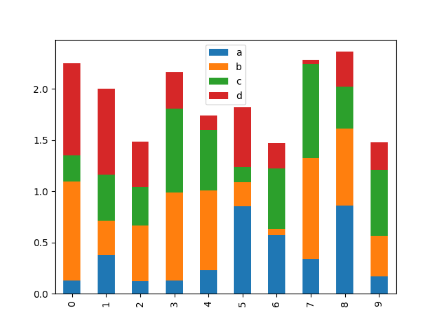
To produce a stacked bar plot, pass stacked=True:
In [23]: df2.plot.bar(stacked=True);
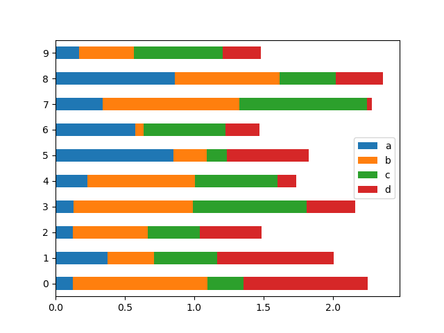
To get horizontal bar plots, use the barh method:
In [24]: df2.plot.barh(stacked=True);
Histograms#
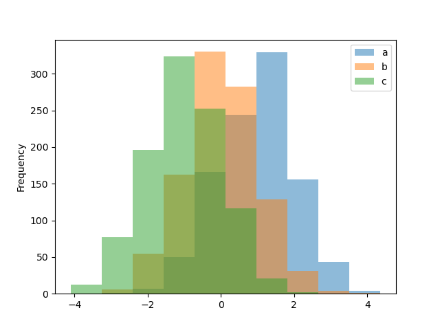
Histograms can be drawn by using the DataFrame.plot.hist() and Series.plot.hist() methods.
In [25]: df4 = pd.DataFrame(
   ....:     {
   ....:         "a": np.random.randn(1000) + 1,
   ....:         "b": np.random.randn(1000),
   ....:         "c": np.random.randn(1000) - 1,
   ....:     },
   ....:     columns=["a", "b", "c"],
   ....: )
   ....:

In [26]: plt.figure();

In [27]: df4.plot.hist(alpha=0.5);
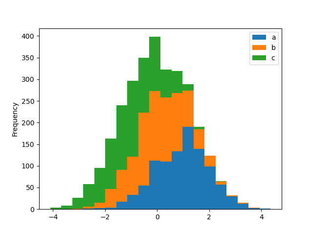
A histogram can be stacked using stacked=True. Bin size can be changed
using the bins keyword.
In [28]: plt.figure();

In [29]: df4.plot.hist(stacked=True, bins=20);
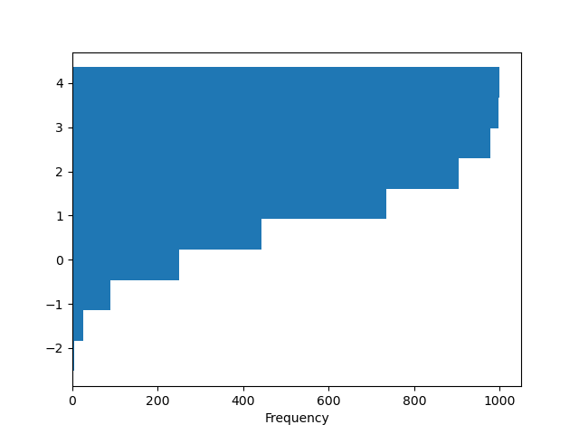
You can pass other keywords supported by matplotlib hist. For example,
horizontal and cumulative histograms can be drawn by
orientation='horizontal' and cumulative=True.
In [30]: plt.figure();

In [31]: df4["a"].plot.hist(orientation="horizontal", cumulative=True);
See the hist method and the
matplotlib hist documentation for more.
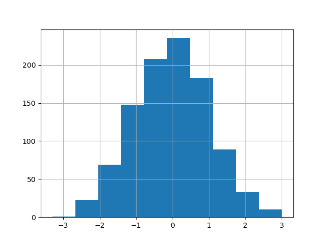
The existing interface DataFrame.hist to plot histogram still can be used.
In [32]: plt.figure();

In [33]: df["A"].diff().hist();
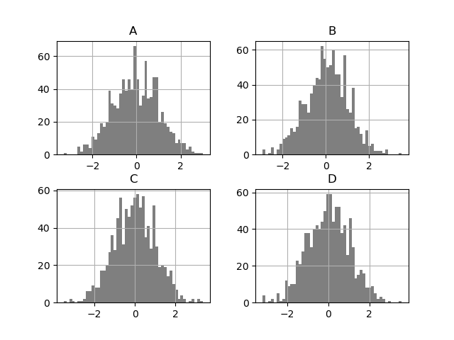
DataFrame.hist() plots the histograms of the columns on multiple
subplots:
In [34]: plt.figure();

In [35]: df.diff().hist(color="k", alpha=0.5, bins=50);
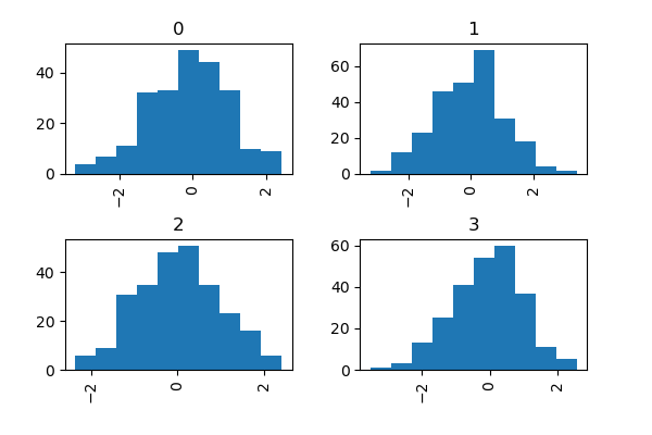
The by keyword can be specified to plot grouped histograms:
In [36]: data = pd.Series(np.random.randn(1000))

In [37]: data.hist(by=np.random.randint(0, 4, 1000), figsize=(6, 4));
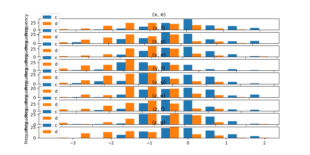
In addition, the by keyword can also be specified in DataFrame.plot.hist().
In [38]: data = pd.DataFrame(
   ....:     {
   ....:         "a": np.random.choice(["x", "y", "z"], 1000),
   ....:         "b": np.random.choice(["e", "f", "g"], 1000),
   ....:         "c": np.random.randn(1000),
   ....:         "d": np.random.randn(1000) - 1,
   ....:     },
   ....: )
   ....:

In [39]: data.plot.hist(by=["a", "b"], figsize=(10, 5));
Box plots#
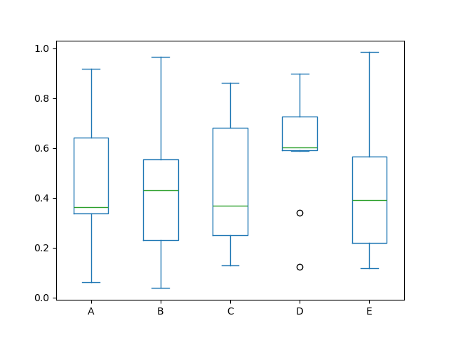
Boxplot can be drawn calling Series.plot.box() and DataFrame.plot.box(),
or DataFrame.boxplot() to visualize the distribution of values within each column.
For instance, here is a boxplot representing five trials of 10 observations of a uniform random variable on [0,1).
In [40]: df = pd.DataFrame(np.random.rand(10, 5), columns=["A", "B", "C", "D", "E"])

In [41]: df.plot.box();
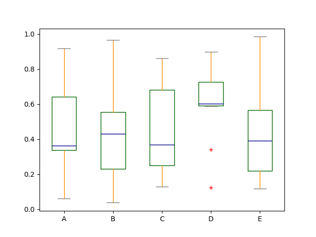
Boxplot can be colorized by passing color keyword. You can pass a dict
whose keys are boxes, whiskers, medians and caps.
If some keys are missing in the dict, default colors are used
for the corresponding artists. Also, boxplot has sym keyword to specify fliers style.
When you pass other type of arguments via color keyword, it will be directly
passed to matplotlib for all the boxes, whiskers, medians and caps
colorization.
The colors are applied to every boxes to be drawn. If you want more complicated colorization, you can get each drawn artists by passing return_type.
In [42]: color = {
   ....:     "boxes": "DarkGreen",
   ....:     "whiskers": "DarkOrange",
   ....:     "medians": "DarkBlue",
   ....:     "caps": "Gray",
   ....: }
   ....:

In [43]: df.plot.box(color=color, sym="r+");
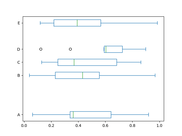
Also, you can pass other keywords supported by matplotlib boxplot.
For example, horizontal and custom-positioned boxplot can be drawn by
vert=False and positions keywords.
In [44]: df.plot.box(vert=False, positions=[1, 4, 5, 6, 8]);
See the boxplot method and the
matplotlib boxplot documentation for more.
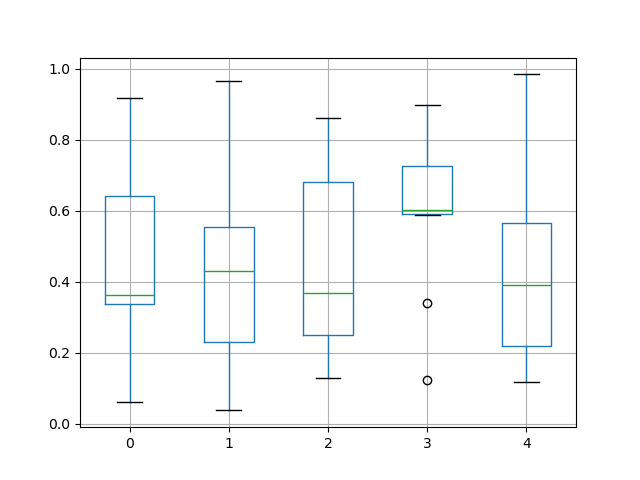
The existing interface DataFrame.boxplot to plot boxplot still can be used.
In [45]: df = pd.DataFrame(np.random.rand(10, 5))

In [46]: plt.figure();

In [47]: bp = df.boxplot()
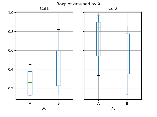
You can create a stratified boxplot using the by keyword argument to create
groupings. For instance,
In [48]: df = pd.DataFrame(np.random.rand(10, 2), columns=["Col1", "Col2"])

In [49]: df["X"] = pd.Series(["A", "A", "A", "A", "A", "B", "B", "B", "B", "B"])

In [50]: plt.figure();

In [51]: bp = df.boxplot(by="X")
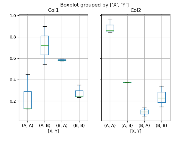
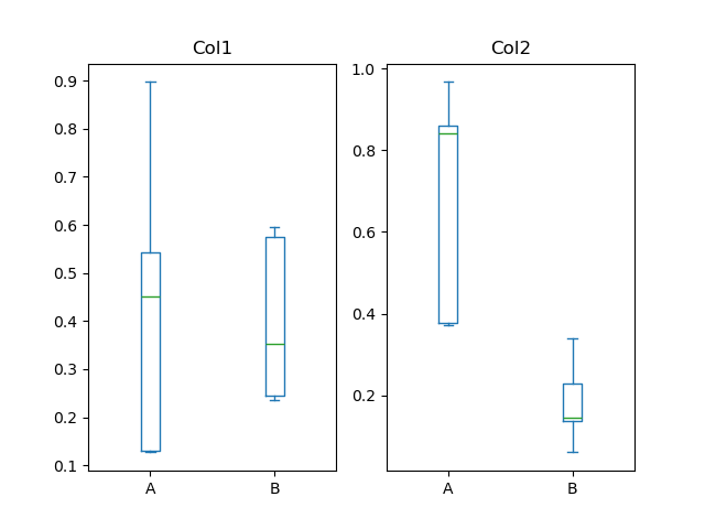
You can also pass a subset of columns to plot, as well as group by multiple columns:
In [52]: df = pd.DataFrame(np.random.rand(10, 3), columns=["Col1", "Col2", "Col3"])

In [53]: df["X"] = pd.Series(["A", "A", "A", "A", "A", "B", "B", "B", "B", "B"])

In [54]: df["Y"] = pd.Series(["A", "B", "A", "B", "A", "B", "A", "B", "A", "B"])

In [55]: plt.figure();

In [56]: bp = df.boxplot(column=["Col1", "Col2"], by=["X", "Y"])
You could also create groupings with DataFrame.plot.box(), for instance:
In [57]: df = pd.DataFrame(np.random.rand(10, 3), columns=["Col1", "Col2", "Col3"])

In [58]: df["X"] = pd.Series(["A", "A", "A", "A", "A", "B", "B", "B", "B", "B"])

In [59]: plt.figure();

In [60]: bp = df.plot.box(column=["Col1", "Col2"], by="X")
In boxplot, the return type can be controlled by the return_type, keyword. The valid choices are {"axes", "dict", "both", None}.
Faceting, created by DataFrame.boxplot with the by
keyword, will affect the output type as well:
|
Faceted |
Output type |
|---|---|---|
|
No |
axes |
|
Yes |
2-D ndarray of axes |
|
No |
axes |
|
Yes |
Series of axes |
|
No |
dict of artists |
|
Yes |
Series of dicts of artists |
|
No |
namedtuple |
|
Yes |
Series of namedtuples |
Groupby.boxplot always returns a Series of return_type.
In [61]: np.random.seed(1234)

In [62]: df_box = pd.DataFrame(np.random.randn(50, 2))

In [63]: df_box["g"] = np.random.choice(["A", "B"], size=50)

In [64]: df_box.loc[df_box["g"] == "B", 1] += 3

In [65]: bp = df_box.boxplot(by="g")
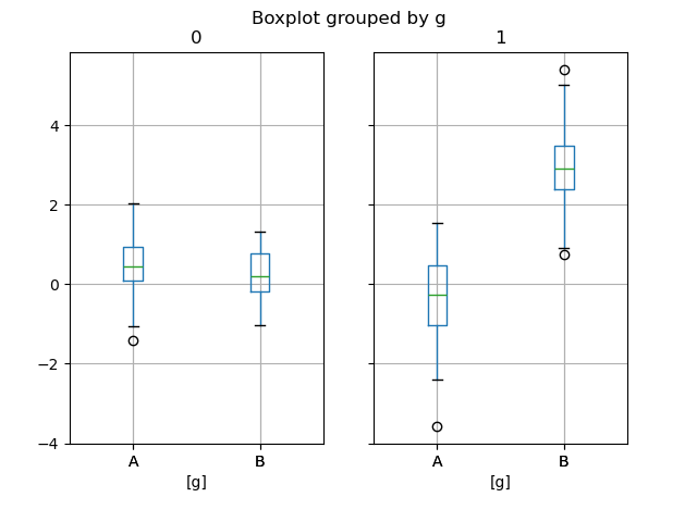
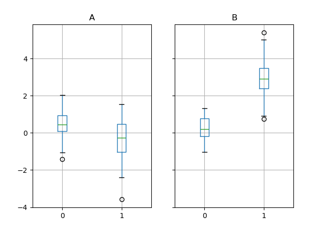
The subplots above are split by the numeric columns first, then the value of
the g column. Below the subplots are first split by the value of g,
then by the numeric columns.
In [66]: bp = df_box.groupby("g").boxplot()
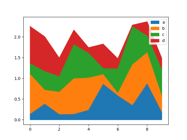
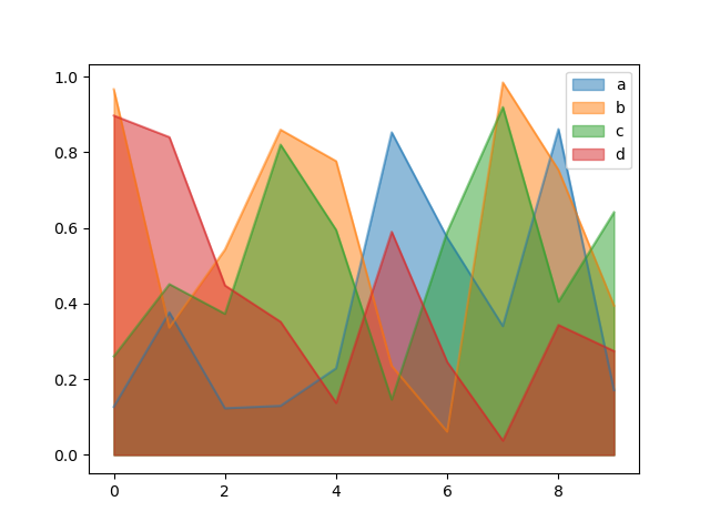
Area plot#
You can create area plots with Series.plot.area() and DataFrame.plot.area().
Area plots are stacked by default. To produce stacked area plot, each column must be either all positive or all negative values.
When input data contains NaN, it will be automatically filled by 0. If you want to drop or fill by different values, use dataframe.dropna() or dataframe.fillna() before calling plot.
In [67]: df = pd.DataFrame(np.random.rand(10, 4), columns=["a", "b", "c", "d"])

In [68]: df.plot.area();
To produce an unstacked plot, pass stacked=False. Alpha value is set to 0.5 unless otherwise specified:
In [69]: df.plot.area(stacked=False);
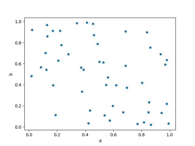
Scatter plot#
Scatter plot can be drawn by using the DataFrame.plot.scatter() method.
Scatter plot requires numeric columns for the x and y axes.
These can be specified by the x and y keywords.
In [70]: df = pd.DataFrame(np.random.rand(50, 4), columns=["a", "b", "c", "d"])

In [71]: df["species"] = pd.Categorical(
   ....:     ["setosa"] * 20 + ["versicolor"] * 20 + ["virginica"] * 10
   ....: )
   ....:

In [72]: df.plot.scatter(x="a", y="b");
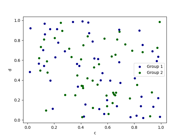
To plot multiple column groups in a single axes, repeat plot method specifying target ax.
It is recommended to specify color and label keywords to distinguish each groups.
In [73]: ax = df.plot.scatter(x="a", y="b", color="DarkBlue", label="Group 1")

In [74]: df.plot.scatter(x="c", y="d", color="DarkGreen", label="Group 2", ax=ax);
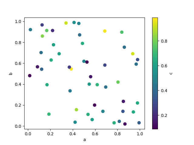
The keyword c may be given as the name of a column to provide colors for
each point:
In [75]: df.plot.scatter(x="a", y="b", c="c", s=50);
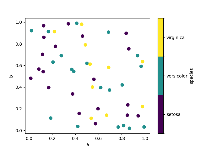
If a categorical column is passed to c, then a discrete colorbar will be produced:
In [76]: df.plot.scatter(x="a", y="b", c="species", cmap="viridis", s=50);
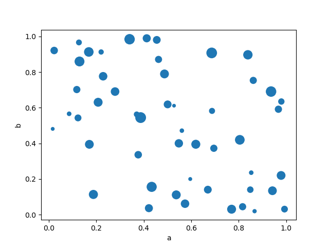
You can pass other keywords supported by matplotlib
scatter. The example below shows a
bubble chart using a column of the DataFrame as the bubble size.
In [77]: df.plot.scatter(x="a", y="b", s=df["c"] * 200);
See the scatter method and the
matplotlib scatter documentation for more.
Hexagonal bin plot#
You can create hexagonal bin plots with DataFrame.plot.hexbin().
Hexbin plots can be a useful alternative to scatter plots if your data are
too dense to plot each point individually.
In [78]: df = pd.DataFrame(np.random.randn(1000, 2), columns=["a", "b"])

In [79]: df["b"] = df["b"] + np.arange(1000)

In [80]: df.plot.hexbin(x="a", y="b", gridsize=25);
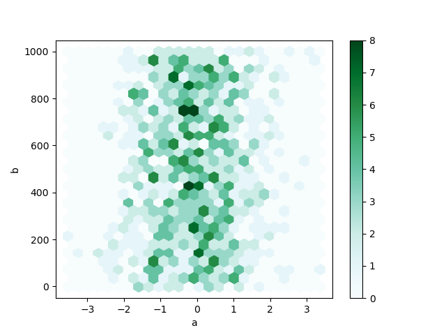
A useful keyword argument is gridsize; it controls the number of hexagons
in the x-direction, and defaults to 100. A larger gridsize means more, smaller
bins.
By default, a histogram of the counts around each (x, y) point is computed.
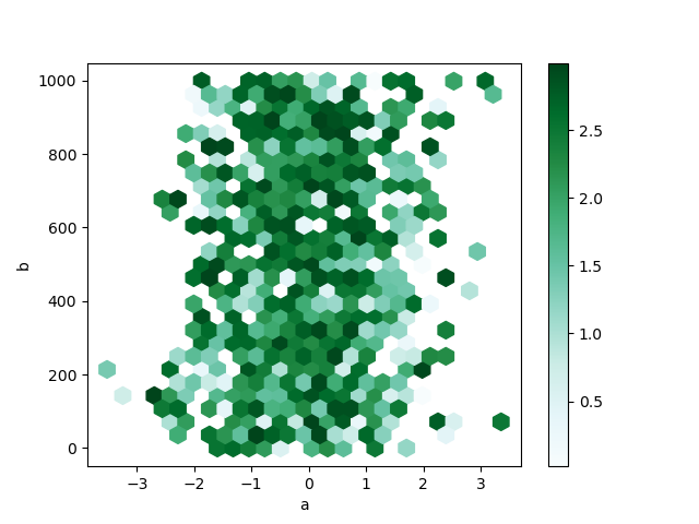
You can specify alternative aggregations by passing values to the C and
reduce_C_function arguments. C specifies the value at each (x, y) point
and reduce_C_function is a function of one argument that reduces all the
values in a bin to a single number (e.g. mean, max, sum, std). In this
example the positions are given by columns a and b, while the value is
given by column z. The bins are aggregated with NumPy’s max function.
In [81]: df = pd.DataFrame(np.random.randn(1000, 2), columns=["a", "b"])

In [82]: df["b"] = df["b"] + np.arange(1000)

In [83]: df["z"] = np.random.uniform(0, 3, 1000)

In [84]: df.plot.hexbin(x="a", y="b", C="z", reduce_C_function=np.max, gridsize=25);
See the hexbin method and the
matplotlib hexbin documentation for more.
Pie plot#
You can create a pie plot with DataFrame.plot.pie() or Series.plot.pie().
If your data includes any NaN, they will be automatically filled with 0.
A ValueError will be raised if there are any negative values in your data.
In [85]: series = pd.Series(3 * np.random.rand(4), index=["a", "b", "c", "d"], name="series")

In [86]: series.plot.pie(figsize=(6, 6));
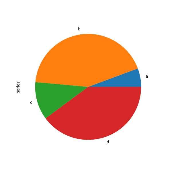
For pie plots it’s best to use square figures, i.e. a figure aspect ratio 1.
You can create the figure with equal width and height, or force the aspect ratio
to be equal after plotting by calling ax.set_aspect('equal') on the returned
axes object.
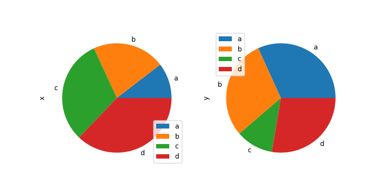
Note that pie plot with DataFrame requires that you either specify a
target column by the y argument or subplots=True. When y is
specified, pie plot of selected column will be drawn. If subplots=True is
specified, pie plots for each column are drawn as subplots. A legend will be
drawn in each pie plots by default; specify legend=False to hide it.
In [87]: df = pd.DataFrame(
   ....:     3 * np.random.rand(4, 2), index=["a", "b", "c", "d"], columns=["x", "y"]
   ....: )
   ....:

In [88]: df.plot.pie(subplots=True, figsize=(8, 4));
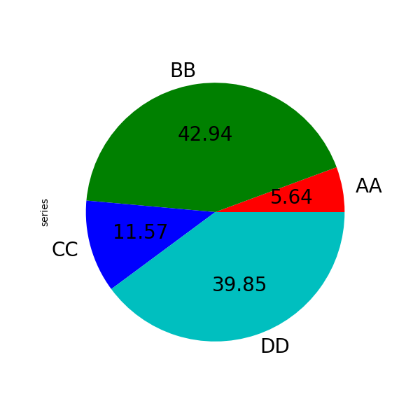
You can use the labels and colors keywords to specify the labels and colors of each wedge.
Warning
Most pandas plots use the label and color arguments (note the lack of “s” on those).
To be consistent with matplotlib.pyplot.pie() you must use labels and colors.
If you want to hide wedge labels, specify labels=None.
If fontsize is specified, the value will be applied to wedge labels.
Also, other keywords supported by matplotlib.pyplot.pie() can be used.
In [89]: series.plot.pie(
   ....:     labels=["AA", "BB", "CC", "DD"],
   ....:     colors=["r", "g", "b", "c"],
   ....:     autopct="%.2f",
   ....:     fontsize=20,
   ....:     figsize=(6, 6),
   ....: );
   ....:
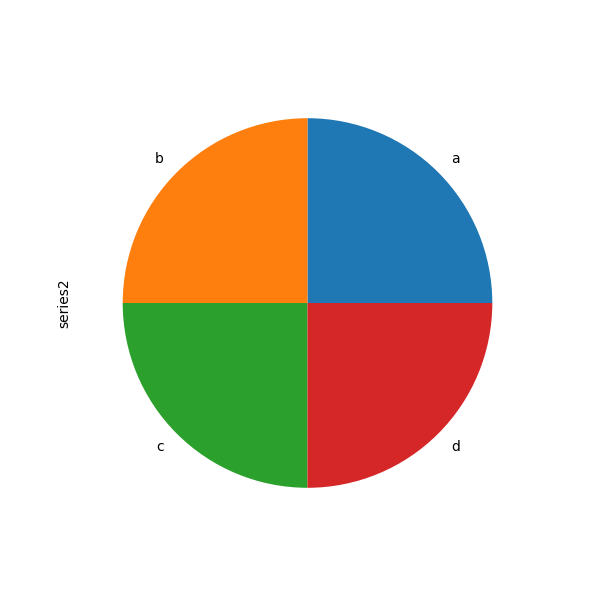
If you pass values whose sum total is less than 1.0 they will be rescaled so that they sum to 1.
In [90]: series = pd.Series([0.1] * 4, index=["a", "b", "c", "d"], name="series2")

In [91]: series.plot.pie(figsize=(6, 6));
See the matplotlib pie documentation for more.
Plotting with missing data#
pandas tries to be pragmatic about plotting DataFrames or Series
that contain missing data. Missing values are dropped, left out, or filled
depending on the plot type.
Plot Type |
NaN Handling |
|---|---|
Line |
Leave gaps at NaNs |
Line (stacked) |
Fill 0’s |
Bar |
Fill 0’s |
Scatter |
Drop NaNs |
Histogram |
Drop NaNs (column-wise) |
Box |
Drop NaNs (column-wise) |
Area |
Fill 0’s |
KDE |
Drop NaNs (column-wise) |
Hexbin |
Drop NaNs |
Pie |
Fill 0’s |
If any of these defaults are not what you want, or if you want to be
explicit about how missing values are handled, consider using
fillna() or dropna()
before plotting.
Plotting tools#
These functions can be imported from pandas.plotting
and take a Series or DataFrame as an argument.
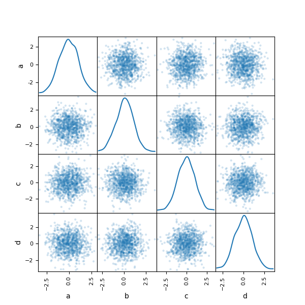
Scatter matrix plot#
You can create a scatter plot matrix using the
scatter_matrix method in pandas.plotting:
In [92]: from pandas.plotting import scatter_matrix

In [93]: df = pd.DataFrame(np.random.randn(1000, 4), columns=["a", "b", "c", "d"])

In [94]: scatter_matrix(df, alpha=0.2, figsize=(6, 6), diagonal="kde");
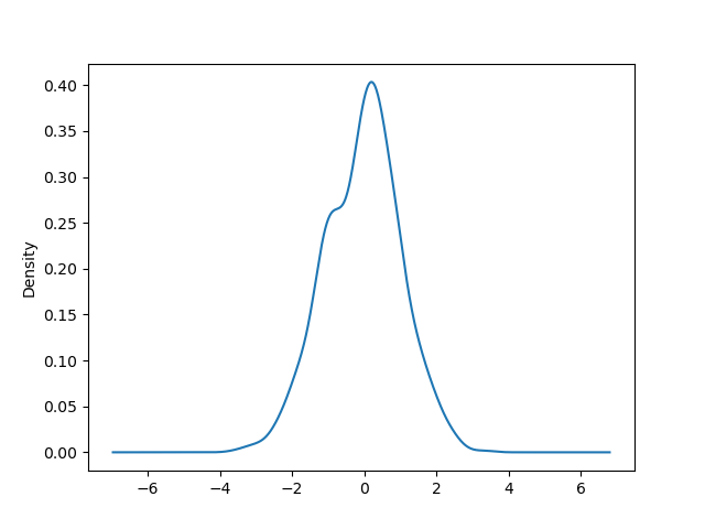
Density plot#
You can create density plots using the Series.plot.kde() and DataFrame.plot.kde() methods.
In [95]: ser = pd.Series(np.random.randn(1000))

In [96]: ser.plot.kde();
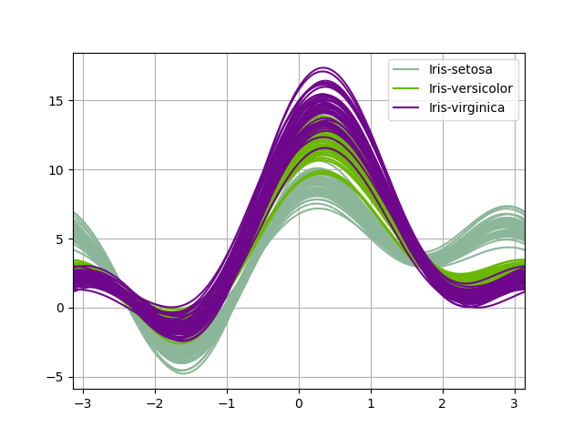
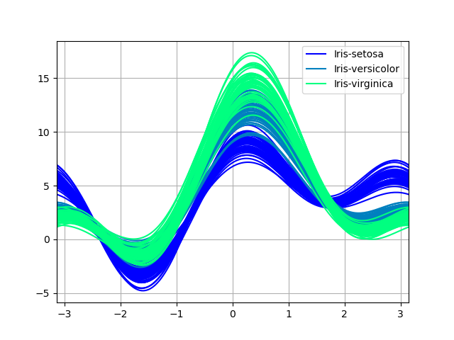
Andrews curves#
Andrews curves allow one to plot multivariate data as a large number of curves that are created using the attributes of samples as coefficients for Fourier series, see the Wikipedia entry for more information. By coloring these curves differently for each class it is possible to visualize data clustering. Curves belonging to samples of the same class will usually be closer together and form larger structures.
Note: The “Iris” dataset is available here.
In [97]: from pandas.plotting import andrews_curves

In [98]: data = pd.read_csv("data/iris.data")

In [99]: plt.figure();

In [100]: andrews_curves(data, "Name");
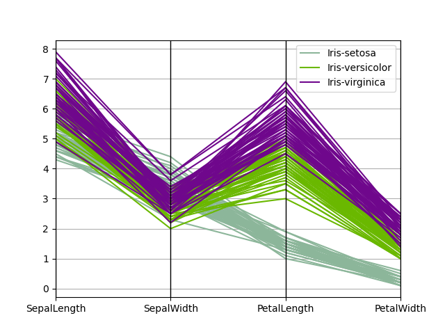
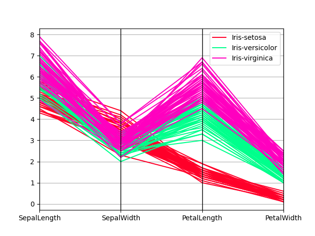
Parallel coordinates#
Parallel coordinates is a plotting technique for plotting multivariate data, see the Wikipedia entry for an introduction. Parallel coordinates allows one to see clusters in data and to estimate other statistics visually. Using parallel coordinates points are represented as connected line segments. Each vertical line represents one attribute. One set of connected line segments represents one data point. Points that tend to cluster will appear closer together.
In [101]: from pandas.plotting import parallel_coordinates

In [102]: data = pd.read_csv("data/iris.data")

In [103]: plt.figure();

In [104]: parallel_coordinates(data, "Name");
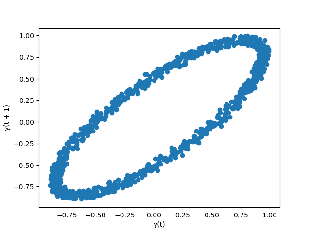
Lag plot#
Lag plots are used to check if a data set or time series is random. Random
data should not exhibit any structure in the lag plot. Non-random structure
implies that the underlying data are not random. The lag argument may
be passed, and when lag=1 the plot is essentially data[:-1] vs.
data[1:].
In [105]: from pandas.plotting import lag_plot

In [106]: plt.figure();

In [107]: spacing = np.linspace(-99 * np.pi, 99 * np.pi, num=1000)

In [108]: data = pd.Series(0.1 * np.random.rand(1000) + 0.9 * np.sin(spacing))

In [109]: lag_plot(data);
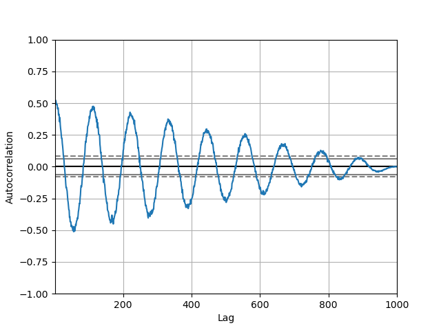
Autocorrelation plot#
Autocorrelation plots are often used for checking randomness in time series. This is done by computing autocorrelations for data values at varying time lags. If time series is random, such autocorrelations should be near zero for any and all time-lag separations. If time series is non-random then one or more of the autocorrelations will be significantly non-zero. The horizontal lines displayed in the plot correspond to 95% and 99% confidence bands. The dashed line is 99% confidence band. See the Wikipedia entry for more about autocorrelation plots.
In [110]: from pandas.plotting import autocorrelation_plot

In [111]: plt.figure();

In [112]: spacing = np.linspace(-9 * np.pi, 9 * np.pi, num=1000)

In [113]: data = pd.Series(0.7 * np.random.rand(1000) + 0.3 * np.sin(spacing))

In [114]: autocorrelation_plot(data);
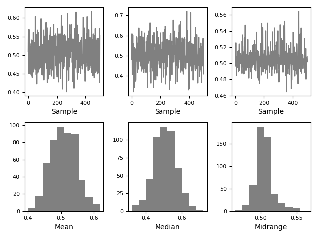
Bootstrap plot#
Bootstrap plots are used to visually assess the uncertainty of a statistic, such as mean, median, midrange, etc. A random subset of a specified size is selected from a data set, the statistic in question is computed for this subset and the process is repeated a specified number of times. Resulting plots and histograms are what constitutes the bootstrap plot.
In [115]: from pandas.plotting import bootstrap_plot

In [116]: data = pd.Series(np.random.rand(1000))

In [117]: bootstrap_plot(data, size=50, samples=500, color="grey");
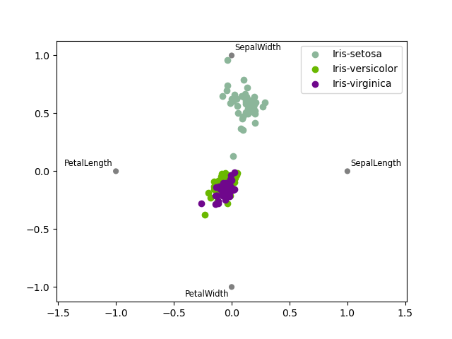
RadViz#
RadViz is a way of visualizing multi-variate data. It is based on a simple spring tension minimization algorithm. Basically you set up a bunch of points in a plane. In our case they are equally spaced on a unit circle. Each point represents a single attribute. You then pretend that each sample in the data set is attached to each of these points by a spring, the stiffness of which is proportional to the numerical value of that attribute (they are normalized to unit interval). The point in the plane, where our sample settles to (where the forces acting on our sample are at an equilibrium) is where a dot representing our sample will be drawn. Depending on which class that sample belongs it will be colored differently. See the R package Radviz for more information.
Note: The “Iris” dataset is available here.
In [118]: from pandas.plotting import radviz

In [119]: data = pd.read_csv("data/iris.data")

In [120]: plt.figure();

In [121]: radviz(data, "Name");
Plot formatting#
Setting the plot style#
From version 1.5 and up, matplotlib offers a range of pre-configured plotting styles. Setting the
style can be used to easily give plots the general look that you want.
Setting the style is as easy as calling matplotlib.style.use(my_plot_style) before
creating your plot. For example you could write matplotlib.style.use('ggplot') for ggplot-style
plots.
You can see the various available style names at matplotlib.style.available and it’s very
easy to try them out.
General plot style arguments#
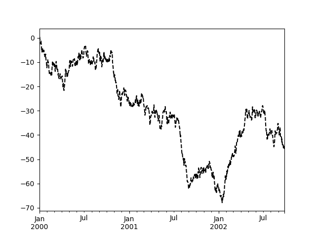
Most plotting methods have a set of keyword arguments that control the layout and formatting of the returned plot:
In [122]: plt.figure();

In [123]: ts.plot(style="k--", label="Series");
For each kind of plot (e.g. line, bar, scatter) any additional arguments
keywords are passed along to the corresponding matplotlib function
(ax.plot(),
ax.bar(),
ax.scatter()). These can be used
to control additional styling, beyond what pandas provides.
Controlling the legend#
You may set the legend argument to False to hide the legend, which is
shown by default.
In [124]: df = pd.DataFrame(np.random.randn(1000, 4), index=ts.index, columns=list("ABCD"))

In [125]: df = df.cumsum()

In [126]: df.plot(legend=False);
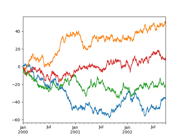
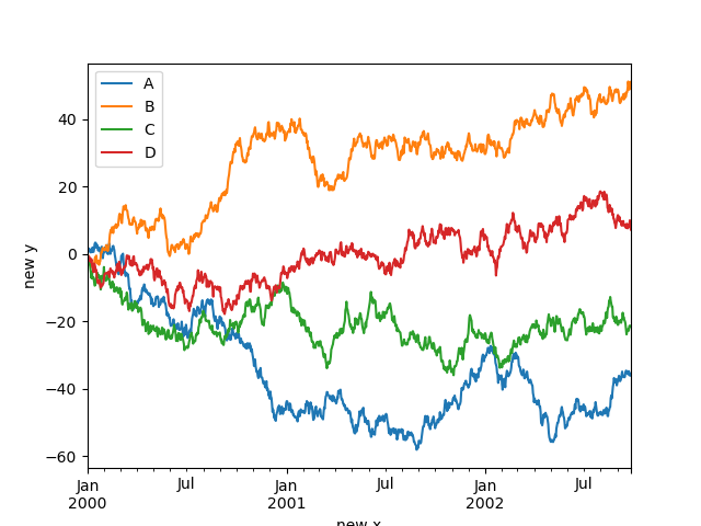
Controlling the labels#
You may set the xlabel and ylabel arguments to give the plot custom labels
for x and y axis. By default, pandas will pick up index name as xlabel, while leaving
it empty for ylabel.
In [127]: df.plot();

In [128]: df.plot(xlabel="new x", ylabel="new y");
Scales#
You may pass logy to get a log-scale Y axis.
In [129]: ts = pd.Series(np.random.randn(1000), index=pd.date_range("1/1/2000", periods=1000))

In [130]: ts = np.exp(ts.cumsum())

In [131]: ts.plot(logy=True);
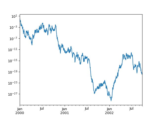
See also the logx and loglog keyword arguments.
Plotting on a secondary y-axis#
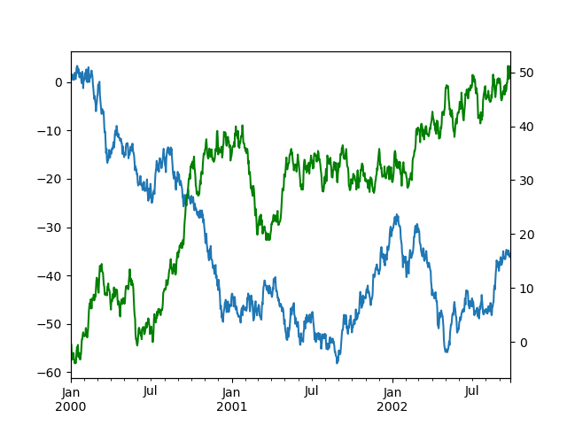
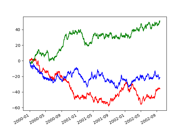
To plot data on a secondary y-axis, use the secondary_y keyword:
In [132]: df["A"].plot();

In [133]: df["B"].plot(secondary_y=True, style="g");
To plot some columns in a DataFrame, give the column names to the secondary_y
keyword:
In [134]: plt.figure();

In [135]: ax = df.plot(secondary_y=["A", "B"])

In [136]: ax.set_ylabel("CD scale");

In [137]: ax.right_ax.set_ylabel("AB scale");
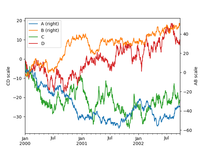
Note that the columns plotted on the secondary y-axis is automatically marked
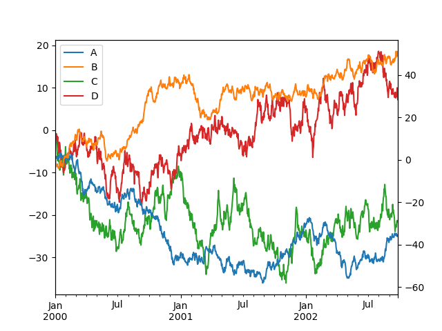
with “(right)” in the legend. To turn off the automatic marking, use the
mark_right=False keyword:
In [138]: plt.figure();

In [139]: df.plot(secondary_y=["A", "B"], mark_right=False);
Custom formatters for timeseries plots#
pandas provides custom formatters for timeseries plots. These change the
formatting of the axis labels for dates and times. By default,
the custom formatters are applied only to plots created by pandas with
DataFrame.plot() or Series.plot(). To have them apply to all
plots, including those made by matplotlib, set the option
pd.options.plotting.matplotlib.register_converters = True or use
pandas.plotting.register_matplotlib_converters().
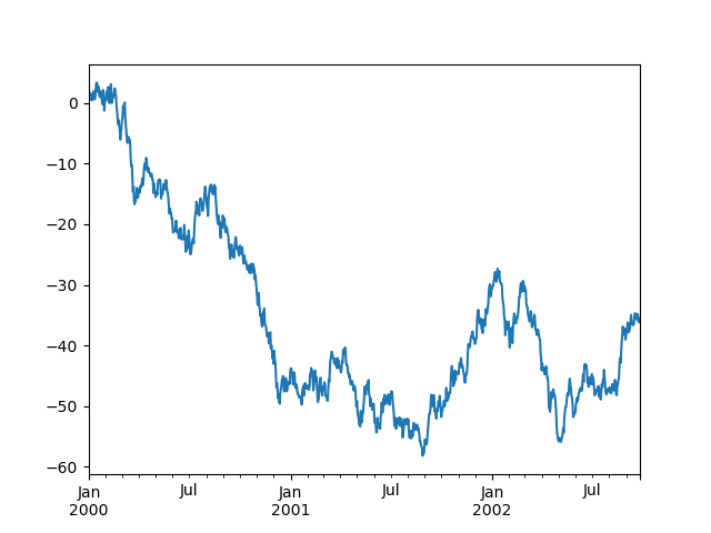
Suppressing tick resolution adjustment#
pandas includes automatic tick resolution adjustment for regular frequency
time-series data. For limited cases where pandas cannot infer the frequency
information (e.g., in an externally created twinx), you can choose to
suppress this behavior for alignment purposes.
Here is the default behavior, notice how the x-axis tick labeling is performed:
In [140]: plt.figure();

In [141]: df["A"].plot();
Using the x_compat parameter, you can suppress this behavior:
In [142]: plt.figure();

In [143]: df["A"].plot(x_compat=True);
If you have more than one plot that needs to be suppressed, the use method
in pandas.plotting.plot_params can be used in a with statement:
In [144]: plt.figure();

In [145]: with pd.plotting.plot_params.use("x_compat", True):
   .....:     df["A"].plot(color="r")
   .....:     df["B"].plot(color="g")
   .....:     df["C"].plot(color="b")
   .....:
Automatic date tick adjustment#
TimedeltaIndex now uses the native matplotlib
tick locator methods, it is useful to call the automatic
date tick adjustment from matplotlib for figures whose ticklabels overlap.
See the autofmt_xdate method and the
matplotlib documentation for more.
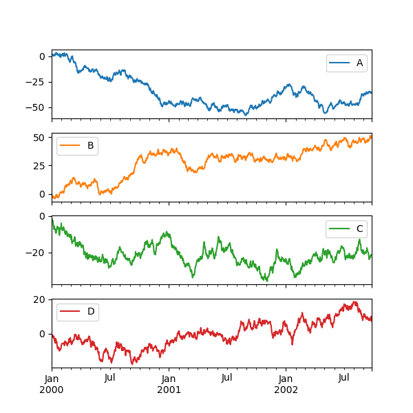
Subplots#
Each Series in a DataFrame can be plotted on a different axis
with the subplots keyword:
In [146]: df.plot(subplots=True, figsize=(6, 6));
Using layout and targeting multiple axes#
The layout of subplots can be specified by the layout keyword. It can accept
(rows, columns). The layout keyword can be used in
hist and boxplot also. If the input is invalid, a ValueError will be raised.
The number of axes which can be contained by rows x columns specified by layout must be
larger than the number of required subplots. If layout can contain more axes than required,
blank axes are not drawn. Similar to a NumPy array’s reshape method, you
can use -1 for one dimension to automatically calculate the number of rows
or columns needed, given the other.
In [147]: df.plot(subplots=True, layout=(2, 3), figsize=(6, 6), sharex=False);
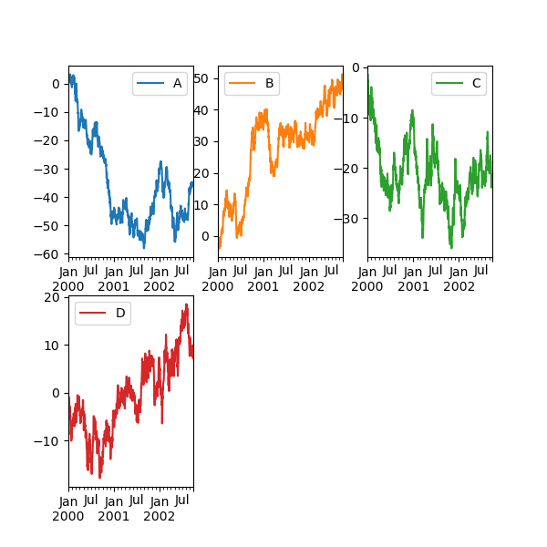
The above example is identical to using:
In [148]: df.plot(subplots=True, layout=(2, -1), figsize=(6, 6), sharex=False);
The required number of columns (3) is inferred from the number of series to plot and the given number of rows (2).
You can pass multiple axes created beforehand as list-like via ax keyword.
This allows more complicated layouts.
The passed axes must be the same number as the subplots being drawn.
When multiple axes are passed via the ax keyword, layout, sharex and sharey keywords
don’t affect to the output. You should explicitly pass sharex=False and sharey=False,
otherwise you will see a warning.
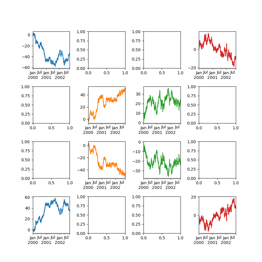
In [149]: fig, axes = plt.subplots(4, 4, figsize=(9, 9))

In [150]: plt.subplots_adjust(wspace=0.5, hspace=0.5)

In [151]: target1 = [axes[0][0], axes[1][1], axes[2][2], axes[3][3]]

In [152]: target2 = [axes[3][0], axes[2][1], axes[1][2], axes[0][3]]

In [153]: df.plot(subplots=True, ax=target1, legend=False, sharex=False, sharey=False);

In [154]: (-df).plot(subplots=True, ax=target2, legend=False, sharex=False, sharey=False);
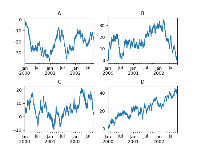
Another option is passing an ax argument to Series.plot() to plot on a particular axis:
In [155]: np.random.seed(123456)

In [156]: ts = pd.Series(np.random.randn(1000), index=pd.date_range("1/1/2000", periods=1000))

In [157]: ts = ts.cumsum()

In [158]: df = pd.DataFrame(np.random.randn(1000, 4), index=ts.index, columns=list("ABCD"))

In [159]: df = df.cumsum()
In [160]: fig, axes = plt.subplots(nrows=2, ncols=2)

In [161]: plt.subplots_adjust(wspace=0.2, hspace=0.5)

In [162]: df["A"].plot(ax=axes[0, 0]);

In [163]: axes[0, 0].set_title("A");

In [164]: df["B"].plot(ax=axes[0, 1]);

In [165]: axes[0, 1].set_title("B");

In [166]: df["C"].plot(ax=axes[1, 0]);

In [167]: axes[1, 0].set_title("C");

In [168]: df["D"].plot(ax=axes[1, 1]);

In [169]: axes[1, 1].set_title("D");
Plotting with error bars#
Plotting with error bars is supported in DataFrame.plot() and Series.plot().
Horizontal and vertical error bars can be supplied to the xerr and yerr keyword arguments to plot(). The error values can be specified using a variety of formats:
As a
DataFrameordictof errors with column names matching thecolumnsattribute of the plottingDataFrameor matching thenameattribute of theSeries.As a
strindicating which of the columns of plottingDataFramecontain the error values.As raw values (
list,tuple, ornp.ndarray). Must be the same length as the plottingDataFrame/Series.
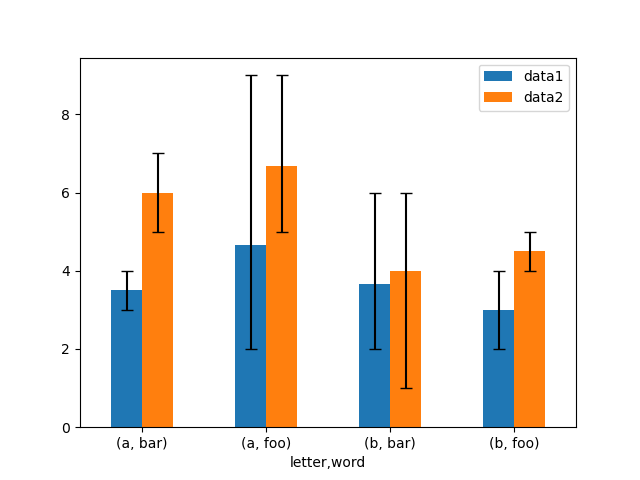
Here is an example of one way to easily plot group means with standard deviations from the raw data.
# Generate the data
In [170]: ix3 = pd.MultiIndex.from_arrays(
   .....:     [
   .....:         ["a", "a", "a", "a", "a", "b", "b", "b", "b", "b"],
   .....:         ["foo", "foo", "foo", "bar", "bar", "foo", "foo", "bar", "bar", "bar"],
   .....:     ],
   .....:     names=["letter", "word"],
   .....: )
   .....:

In [171]: df3 = pd.DataFrame(
   .....:     {
   .....:         "data1": [9, 3, 2, 4, 3, 2, 4, 6, 3, 2],
   .....:         "data2": [9, 6, 5, 7, 5, 4, 5, 6, 5, 1],
   .....:     },
   .....:     index=ix3,
   .....: )
   .....:

# Group by index labels and take the means and standard deviations
# for each group
In [172]: gp3 = df3.groupby(level=("letter", "word"))

In [173]: means = gp3.mean()

In [174]: errors = gp3.std()

In [175]: means
Out[175]:
                data1     data2
letter word
a      bar   3.500000  6.000000
       foo   4.666667  6.666667
b      bar   3.666667  4.000000
       foo   3.000000  4.500000

In [176]: errors
Out[176]:
                data1     data2
letter word
a      bar   0.707107  1.414214
       foo   3.785939  2.081666
b      bar   2.081666  2.645751
       foo   1.414214  0.707107

# Plot
In [177]: fig, ax = plt.subplots()

In [178]: means.plot.bar(yerr=errors, ax=ax, capsize=4, rot=0);
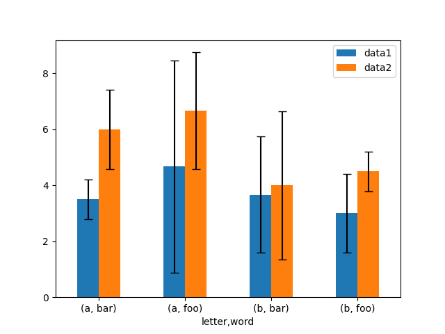
Asymmetrical error bars are also supported, however raw error values must be provided in this case. For a N length Series, a 2xN array should be provided indicating lower and upper (or left and right) errors. For a MxN DataFrame, asymmetrical errors should be in a Mx2xN array.
Here is an example of one way to plot the min/max range using asymmetrical error bars.
In [179]: mins = gp3.min()

In [180]: maxs = gp3.max()

# errors should be positive, and defined in the order of lower, upper
In [181]: errors = [[means[c] - mins[c], maxs[c] - means[c]] for c in df3.columns]

# Plot
In [182]: fig, ax = plt.subplots()

In [183]: means.plot.bar(yerr=errors, ax=ax, capsize=4, rot=0);
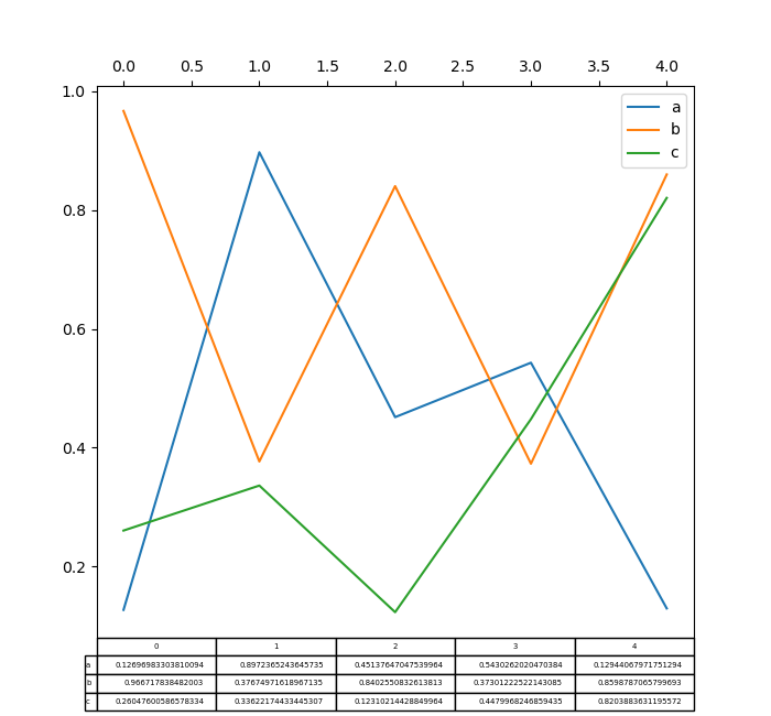
Plotting tables#
Plotting with matplotlib table is now supported in DataFrame.plot() and Series.plot() with a table keyword. The table keyword can accept bool, DataFrame or Series. The simple way to draw a table is to specify table=True. Data will be transposed to meet matplotlib’s default layout.
In [184]: np.random.seed(123456)

In [185]: fig, ax = plt.subplots(1, 1, figsize=(7, 6.5))

In [186]: df = pd.DataFrame(np.random.rand(5, 3), columns=["a", "b", "c"])

In [187]: ax.xaxis.tick_top()  # Display x-axis ticks on top.

In [188]: df.plot(table=True, ax=ax);
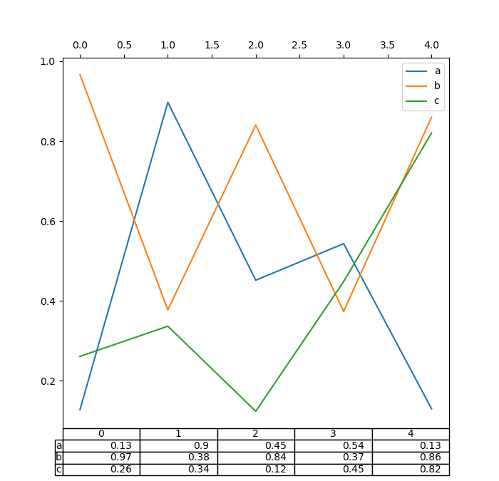
Also, you can pass a different DataFrame or Series to the
table keyword. The data will be drawn as displayed in print method
(not transposed automatically). If required, it should be transposed manually
as seen in the example below.
In [189]: fig, ax = plt.subplots(1, 1, figsize=(7, 6.75))

In [190]: ax.xaxis.tick_top()  # Display x-axis ticks on top.

In [191]: df.plot(table=np.round(df.T, 2), ax=ax);
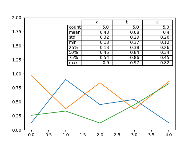
There also exists a helper function pandas.plotting.table, which creates a
table from DataFrame or Series, and adds it to an
matplotlib.Axes instance. This function can accept keywords which the
matplotlib table has.
In [192]: from pandas.plotting import table

In [193]: fig, ax = plt.subplots(1, 1)

In [194]: table(ax, np.round(df.describe(), 2), loc="upper right", colWidths=[0.2, 0.2, 0.2]);

In [195]: df.plot(ax=ax, ylim=(0, 2), legend=None);
Note: You can get table instances on the axes using axes.tables property for further decorations. See the matplotlib table documentation for more.
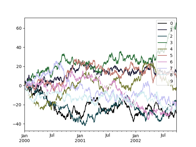
Colormaps#
A potential issue when plotting a large number of columns is that it can be
difficult to distinguish some series due to repetition in the default colors. To
remedy this, DataFrame plotting supports the use of the colormap argument,
which accepts either a Matplotlib colormap
or a string that is a name of a colormap registered with Matplotlib. A
visualization of the default matplotlib colormaps is available here.
As matplotlib does not directly support colormaps for line-based plots, the
colors are selected based on an even spacing determined by the number of columns
in the DataFrame. There is no consideration made for background color, so some
colormaps will produce lines that are not easily visible.
To use the cubehelix colormap, we can pass colormap='cubehelix'.
In [196]: np.random.seed(123456)

In [197]: df = pd.DataFrame(np.random.randn(1000, 10), index=ts.index)

In [198]: df = df.cumsum()

In [199]: plt.figure();

In [200]: df.plot(colormap="cubehelix");
Alternatively, we can pass the colormap itself:
In [201]: from matplotlib import cm

In [202]: plt.figure();

In [203]: df.plot(colormap=cm.cubehelix);

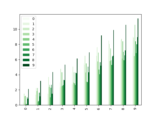
Colormaps can also be used other plot types, like bar charts:
In [204]: np.random.seed(123456)

In [205]: dd = pd.DataFrame(np.random.randn(10, 10)).map(abs)

In [206]: dd = dd.cumsum()

In [207]: plt.figure();

In [208]: dd.plot.bar(colormap="Greens");
Parallel coordinates charts:
In [209]: plt.figure();

In [210]: parallel_coordinates(data, "Name", colormap="gist_rainbow");
Andrews curves charts:
In [211]: plt.figure();

In [212]: andrews_curves(data, "Name", colormap="winter");
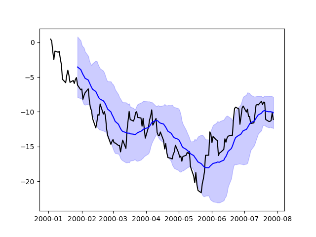
Plotting directly with Matplotlib#
In some situations it may still be preferable or necessary to prepare plots
directly with matplotlib, for instance when a certain type of plot or
customization is not (yet) supported by pandas. Series and DataFrame
objects behave like arrays and can therefore be passed directly to
matplotlib functions without explicit casts.
pandas also automatically registers formatters and locators that recognize date indices, thereby extending date and time support to practically all plot types available in matplotlib. Although this formatting does not provide the same level of refinement you would get when plotting via pandas, it can be faster when plotting a large number of points.
In [213]: np.random.seed(123456)

In [214]: price = pd.Series(
   .....:     np.random.randn(150).cumsum(),
   .....:     index=pd.date_range("2000-1-1", periods=150, freq="B"),
   .....: )
   .....:

In [215]: ma = price.rolling(20).mean()

In [216]: mstd = price.rolling(20).std()

In [217]: plt.figure();

In [218]: plt.plot(price.index, price, "k");

In [219]: plt.plot(ma.index, ma, "b");

In [220]: plt.fill_between(mstd.index, ma - 2 * mstd, ma + 2 * mstd, color="b", alpha=0.2);
Plotting backends#
pandas can be extended with third-party plotting backends. The main idea is letting users select a plotting backend different than the provided one based on Matplotlib.
This can be done by passing ‘backend.module’ as the argument backend in plot
function. For example:
>>> Series([1, 2, 3]).plot(backend="backend.module")
Alternatively, you can also set this option globally, do you don’t need to specify
the keyword in each plot call. For example:
>>> pd.set_option("plotting.backend", "backend.module")
>>> pd.Series([1, 2, 3]).plot()
Or:
>>> pd.options.plotting.backend = "backend.module"
>>> pd.Series([1, 2, 3]).plot()
This would be more or less equivalent to:
>>> import backend.module
>>> backend.module.plot(pd.Series([1, 2, 3]))
The backend module can then use other visualization tools (Bokeh, Altair, hvplot,…) to generate the plots. Some libraries implementing a backend for pandas are listed on the ecosystem page.
Developers guide can be found at https://pandas.pydata.org/docs/dev/development/extending.html#plotting-backends