

10 minutes to pandas#
This is a short introduction to pandas, geared mainly for new users. You can see more complex recipes in the Cookbook.
Customarily, we import as follows:
In [1]: import numpy as np

In [2]: import pandas as pd
Basic data structures in pandas#
pandas provides two types of classes for handling data:
Object creation#
See the Intro to data structures section.
Creating a Series by passing a list of values, letting pandas create
a default RangeIndex.
In [3]: s = pd.Series([1, 3, 5, np.nan, 6, 8])

In [4]: s
Out[4]:
0    1.0
1    3.0
2    5.0
3    NaN
4    6.0
5    8.0
dtype: float64
Creating a DataFrame by passing a NumPy array with a datetime index using date_range()
and labeled columns:
In [5]: dates = pd.date_range("20130101", periods=6)

In [6]: dates
Out[6]:
DatetimeIndex(['2013-01-01', '2013-01-02', '2013-01-03', '2013-01-04',
               '2013-01-05', '2013-01-06'],
              dtype='datetime64[us]', freq='D')

In [7]: df = pd.DataFrame(np.random.randn(6, 4), index=dates, columns=list("ABCD"))

In [8]: df
Out[8]:
                   A         B         C         D
2013-01-01  0.469112 -0.282863 -1.509059 -1.135632
2013-01-02  1.212112 -0.173215  0.119209 -1.044236
2013-01-03 -0.861849 -2.104569 -0.494929  1.071804
2013-01-04  0.721555 -0.706771 -1.039575  0.271860
2013-01-05 -0.424972  0.567020  0.276232 -1.087401
2013-01-06 -0.673690  0.113648 -1.478427  0.524988
Creating a DataFrame by passing a dictionary of objects where the keys are the column
labels and the values are the column values.
In [9]: df2 = pd.DataFrame(
   ...:     {
   ...:         "A": 1.0,
   ...:         "B": pd.Timestamp("20130102"),
   ...:         "C": pd.Series(1, index=list(range(4)), dtype="float32"),
   ...:         "D": np.array([3] * 4, dtype="int32"),
   ...:         "E": pd.Categorical(["test", "train", "test", "train"]),
   ...:         "F": "foo",
   ...:     }
   ...: )
   ...:

In [10]: df2
Out[10]:
     A          B    C  D      E    F
0  1.0 2013-01-02  1.0  3   test  foo
1  1.0 2013-01-02  1.0  3  train  foo
2  1.0 2013-01-02  1.0  3   test  foo
3  1.0 2013-01-02  1.0  3  train  foo
The columns of the resulting DataFrame have different
dtypes:
In [11]: df2.dtypes
Out[11]:
A           float64
B    datetime64[us]
C           float32
D             int32
E          category
F               str
dtype: object
If you’re using IPython, tab completion for column names (as well as public attributes) is automatically enabled. Here’s a subset of the attributes that will be completed:
In [12]: df2.<TAB>  # noqa: E225, E999
df2.A                  df2.bool
df2.abs                df2.boxplot
df2.add                df2.C
df2.add_prefix         df2.clip
df2.add_suffix         df2.columns
df2.align              df2.copy
df2.all                df2.count
df2.any                df2.combine
df2.append             df2.D
df2.apply              df2.describe
df2.B                  df2.duplicated
df2.diff
As you can see, the columns A, B, C, and D are automatically
tab completed. E and F are there as well; the rest of the attributes have been
truncated for brevity.
Viewing data#
See the Essential basic functionality section.
Use DataFrame.head() and DataFrame.tail() to view the top and bottom rows of the frame
respectively:
In [13]: df.head()
Out[13]:
                   A         B         C         D
2013-01-01  0.469112 -0.282863 -1.509059 -1.135632
2013-01-02  1.212112 -0.173215  0.119209 -1.044236
2013-01-03 -0.861849 -2.104569 -0.494929  1.071804
2013-01-04  0.721555 -0.706771 -1.039575  0.271860
2013-01-05 -0.424972  0.567020  0.276232 -1.087401

In [14]: df.tail(3)
Out[14]:
                   A         B         C         D
2013-01-04  0.721555 -0.706771 -1.039575  0.271860
2013-01-05 -0.424972  0.567020  0.276232 -1.087401
2013-01-06 -0.673690  0.113648 -1.478427  0.524988
Display the DataFrame.index or DataFrame.columns:
In [15]: df.index
Out[15]:
DatetimeIndex(['2013-01-01', '2013-01-02', '2013-01-03', '2013-01-04',
               '2013-01-05', '2013-01-06'],
              dtype='datetime64[us]', freq='D')

In [16]: df.columns
Out[16]: Index(['A', 'B', 'C', 'D'], dtype='str')
Return a NumPy representation of the underlying data with DataFrame.to_numpy()
without the index or column labels:
In [17]: df.to_numpy()
Out[17]:
array([[ 0.4691, -0.2829, -1.5091, -1.1356],
       [ 1.2121, -0.1732,  0.1192, -1.0442],
       [-0.8618, -2.1046, -0.4949,  1.0718],
       [ 0.7216, -0.7068, -1.0396,  0.2719],
       [-0.425 ,  0.567 ,  0.2762, -1.0874],
       [-0.6737,  0.1136, -1.4784,  0.525 ]])
Note
NumPy arrays have one dtype for the entire array while pandas DataFrames
have one dtype per column. When you call DataFrame.to_numpy(), pandas will
find the NumPy dtype that can hold all of the dtypes in the DataFrame.
If the common data type is object, DataFrame.to_numpy() will require
copying data.
In [18]: df2.dtypes
Out[18]:
A           float64
B    datetime64[us]
C           float32
D             int32
E          category
F               str
dtype: object

In [19]: df2.to_numpy()
Out[19]:
array([[1.0, Timestamp('2013-01-02 00:00:00'), 1.0, 3, 'test', 'foo'],
       [1.0, Timestamp('2013-01-02 00:00:00'), 1.0, 3, 'train', 'foo'],
       [1.0, Timestamp('2013-01-02 00:00:00'), 1.0, 3, 'test', 'foo'],
       [1.0, Timestamp('2013-01-02 00:00:00'), 1.0, 3, 'train', 'foo']],
      dtype=object)
describe() shows a quick statistic summary of your data:
In [20]: df.describe()
Out[20]:
              A         B         C         D
count  6.000000  6.000000  6.000000  6.000000
mean   0.073711 -0.431125 -0.687758 -0.233103
std    0.843157  0.922818  0.779887  0.973118
min   -0.861849 -2.104569 -1.509059 -1.135632
25%   -0.611510 -0.600794 -1.368714 -1.076610
50%    0.022070 -0.228039 -0.767252 -0.386188
75%    0.658444  0.041933 -0.034326  0.461706
max    1.212112  0.567020  0.276232  1.071804
Transposing your data:
In [21]: df.T
Out[21]:
   2013-01-01  2013-01-02  2013-01-03  2013-01-04  2013-01-05  2013-01-06
A    0.469112    1.212112   -0.861849    0.721555   -0.424972   -0.673690
B   -0.282863   -0.173215   -2.104569   -0.706771    0.567020    0.113648
C   -1.509059    0.119209   -0.494929   -1.039575    0.276232   -1.478427
D   -1.135632   -1.044236    1.071804    0.271860   -1.087401    0.524988
DataFrame.sort_index() sorts by an axis:
In [22]: df.sort_index(axis=1, ascending=False)
Out[22]:
                   D         C         B         A
2013-01-01 -1.135632 -1.509059 -0.282863  0.469112
2013-01-02 -1.044236  0.119209 -0.173215  1.212112
2013-01-03  1.071804 -0.494929 -2.104569 -0.861849
2013-01-04  0.271860 -1.039575 -0.706771  0.721555
2013-01-05 -1.087401  0.276232  0.567020 -0.424972
2013-01-06  0.524988 -1.478427  0.113648 -0.673690
DataFrame.sort_values() sorts by values:
In [23]: df.sort_values(by="B")
Out[23]:
                   A         B         C         D
2013-01-03 -0.861849 -2.104569 -0.494929  1.071804
2013-01-04  0.721555 -0.706771 -1.039575  0.271860
2013-01-01  0.469112 -0.282863 -1.509059 -1.135632
2013-01-02  1.212112 -0.173215  0.119209 -1.044236
2013-01-06 -0.673690  0.113648 -1.478427  0.524988
2013-01-05 -0.424972  0.567020  0.276232 -1.087401
Selection#
Note
While standard Python / NumPy expressions for selecting and setting are
intuitive and come in handy for interactive work, for production code, we
recommend the optimized pandas data access methods, DataFrame.at(), DataFrame.iat(),
DataFrame.loc() and DataFrame.iloc().
See the indexing documentation Indexing and Selecting Data and MultiIndex / Advanced Indexing.
Getitem ([])#
For a DataFrame, passing a single label selects a column and
yields a Series:
In [24]: df["A"]
Out[24]:
2013-01-01    0.469112
2013-01-02    1.212112
2013-01-03   -0.861849
2013-01-04    0.721555
2013-01-05   -0.424972
2013-01-06   -0.673690
Freq: D, Name: A, dtype: float64
If the label only contains letters, numbers, and underscores, you can alternatively use the column name attribute:
In [25]: df.A
Out[25]:
2013-01-01    0.469112
2013-01-02    1.212112
2013-01-03   -0.861849
2013-01-04    0.721555
2013-01-05   -0.424972
2013-01-06   -0.673690
Freq: D, Name: A, dtype: float64
Passing a list of column labels selects multiple columns, which can be useful for getting a subset/rearranging:
In [26]: df[["B", "A"]]
Out[26]:
                   B         A
2013-01-01 -0.282863  0.469112
2013-01-02 -0.173215  1.212112
2013-01-03 -2.104569 -0.861849
2013-01-04 -0.706771  0.721555
2013-01-05  0.567020 -0.424972
2013-01-06  0.113648 -0.673690
For a DataFrame, passing a slice : selects matching rows:
In [27]: df[0:3]
Out[27]:
                   A         B         C         D
2013-01-01  0.469112 -0.282863 -1.509059 -1.135632
2013-01-02  1.212112 -0.173215  0.119209 -1.044236
2013-01-03 -0.861849 -2.104569 -0.494929  1.071804

In [28]: df["20130102":"20130104"]
Out[28]:
                   A         B         C         D
2013-01-02  1.212112 -0.173215  0.119209 -1.044236
2013-01-03 -0.861849 -2.104569 -0.494929  1.071804
2013-01-04  0.721555 -0.706771 -1.039575  0.271860
Selection by label#
See more in Selection by Label using DataFrame.loc() or DataFrame.at().
Selecting a row matching a label:
In [29]: df.loc[dates[0]]
Out[29]:
A    0.469112
B   -0.282863
C   -1.509059
D   -1.135632
Name: 2013-01-01 00:00:00, dtype: float64
Selecting all rows (:) with a select column labels:
In [30]: df.loc[:, ["A", "B"]]
Out[30]:
                   A         B
2013-01-01  0.469112 -0.282863
2013-01-02  1.212112 -0.173215
2013-01-03 -0.861849 -2.104569
2013-01-04  0.721555 -0.706771
2013-01-05 -0.424972  0.567020
2013-01-06 -0.673690  0.113648
For label slicing, both endpoints are included:
In [31]: df.loc["20130102":"20130104", ["A", "B"]]
Out[31]:
                   A         B
2013-01-02  1.212112 -0.173215
2013-01-03 -0.861849 -2.104569
2013-01-04  0.721555 -0.706771
Selecting a single row and column label returns a scalar:
In [32]: df.loc[dates[0], "A"]
Out[32]: np.float64(0.4691122999071863)
For getting fast access to a scalar (equivalent to the prior method):
In [33]: df.at[dates[0], "A"]
Out[33]: np.float64(0.4691122999071863)
Selection by position#
See more in Selection by Position using DataFrame.iloc() or DataFrame.iat().
Select via the position of the passed integers:
In [34]: df.iloc[3]
Out[34]:
A    0.721555
B   -0.706771
C   -1.039575
D    0.271860
Name: 2013-01-04 00:00:00, dtype: float64
Integer slices acts similar to NumPy/Python:
In [35]: df.iloc[3:5, 0:2]
Out[35]:
                   A         B
2013-01-04  0.721555 -0.706771
2013-01-05 -0.424972  0.567020
Lists of integer position locations:
In [36]: df.iloc[[1, 2, 4], [0, 2]]
Out[36]:
                   A         C
2013-01-02  1.212112  0.119209
2013-01-03 -0.861849 -0.494929
2013-01-05 -0.424972  0.276232
For slicing rows explicitly:
In [37]: df.iloc[1:3, :]
Out[37]:
                   A         B         C         D
2013-01-02  1.212112 -0.173215  0.119209 -1.044236
2013-01-03 -0.861849 -2.104569 -0.494929  1.071804
For slicing columns explicitly:
In [38]: df.iloc[:, 1:3]
Out[38]:
                   B         C
2013-01-01 -0.282863 -1.509059
2013-01-02 -0.173215  0.119209
2013-01-03 -2.104569 -0.494929
2013-01-04 -0.706771 -1.039575
2013-01-05  0.567020  0.276232
2013-01-06  0.113648 -1.478427
For getting a value explicitly:
In [39]: df.iloc[1, 1]
Out[39]: np.float64(-0.17321464905330858)
For getting fast access to a scalar (equivalent to the prior method):
In [40]: df.iat[1, 1]
Out[40]: np.float64(-0.17321464905330858)
Boolean indexing#
Select rows where df.A is greater than 0.
In [41]: df[df["A"] > 0]
Out[41]:
                   A         B         C         D
2013-01-01  0.469112 -0.282863 -1.509059 -1.135632
2013-01-02  1.212112 -0.173215  0.119209 -1.044236
2013-01-04  0.721555 -0.706771 -1.039575  0.271860
Selecting values from a DataFrame where a boolean condition is met:
In [42]: df[df > 0]
Out[42]:
                   A         B         C         D
2013-01-01  0.469112       NaN       NaN       NaN
2013-01-02  1.212112       NaN  0.119209       NaN
2013-01-03       NaN       NaN       NaN  1.071804
2013-01-04  0.721555       NaN       NaN  0.271860
2013-01-05       NaN  0.567020  0.276232       NaN
2013-01-06       NaN  0.113648       NaN  0.524988
Using isin() method for filtering:
In [43]: df2 = df.copy()

In [44]: df2["E"] = ["one", "one", "two", "three", "four", "three"]

In [45]: df2
Out[45]:
                   A         B         C         D      E
2013-01-01  0.469112 -0.282863 -1.509059 -1.135632    one
2013-01-02  1.212112 -0.173215  0.119209 -1.044236    one
2013-01-03 -0.861849 -2.104569 -0.494929  1.071804    two
2013-01-04  0.721555 -0.706771 -1.039575  0.271860  three
2013-01-05 -0.424972  0.567020  0.276232 -1.087401   four
2013-01-06 -0.673690  0.113648 -1.478427  0.524988  three

In [46]: df2[df2["E"].isin(["two", "four"])]
Out[46]:
                   A         B         C         D     E
2013-01-03 -0.861849 -2.104569 -0.494929  1.071804   two
2013-01-05 -0.424972  0.567020  0.276232 -1.087401  four
Setting#
Setting a new column automatically aligns the data by the indexes:
In [47]: s1 = pd.Series(
   ....:    [1, 2, 3, 4, 5, 6],
   ....:    index=pd.date_range("20130102", periods=6))
   ....:

In [48]: s1
Out[48]:
2013-01-02    1
2013-01-03    2
2013-01-04    3
2013-01-05    4
2013-01-06    5
2013-01-07    6
Freq: D, dtype: int64

In [49]: df["F"] = s1
Setting values by label:
In [50]: df.at[dates[0], "A"] = 0
Setting values by position:
In [51]: df.iat[0, 1] = 0
Setting by assigning with a NumPy array:
In [52]: df.loc[:, "D"] = np.array([5] * len(df))
The result of the prior setting operations:
In [53]: df
Out[53]:
                   A         B         C    D    F
2013-01-01  0.000000  0.000000 -1.509059  5.0  NaN
2013-01-02  1.212112 -0.173215  0.119209  5.0  1.0
2013-01-03 -0.861849 -2.104569 -0.494929  5.0  2.0
2013-01-04  0.721555 -0.706771 -1.039575  5.0  3.0
2013-01-05 -0.424972  0.567020  0.276232  5.0  4.0
2013-01-06 -0.673690  0.113648 -1.478427  5.0  5.0
A where operation with setting:
In [54]: df2 = df.copy()

In [55]: df2[df2 > 0] = -df2

In [56]: df2
Out[56]:
                   A         B         C    D    F
2013-01-01  0.000000  0.000000 -1.509059 -5.0  NaN
2013-01-02 -1.212112 -0.173215 -0.119209 -5.0 -1.0
2013-01-03 -0.861849 -2.104569 -0.494929 -5.0 -2.0
2013-01-04 -0.721555 -0.706771 -1.039575 -5.0 -3.0
2013-01-05 -0.424972 -0.567020 -0.276232 -5.0 -4.0
2013-01-06 -0.673690 -0.113648 -1.478427 -5.0 -5.0
Missing data#
For NumPy data types, np.nan represents missing data. It is by
default not included in computations. See the Missing Data section.
Reindexing allows you to change/add/delete the index on a specified axis. This returns a copy of the data:
In [57]: df1 = df.reindex(index=dates[0:4], columns=list(df.columns) + ["E"])

In [58]: df1.loc[dates[0] : dates[1], "E"] = 1

In [59]: df1
Out[59]:
                   A         B         C    D    F    E
2013-01-01  0.000000  0.000000 -1.509059  5.0  NaN  1.0
2013-01-02  1.212112 -0.173215  0.119209  5.0  1.0  1.0
2013-01-03 -0.861849 -2.104569 -0.494929  5.0  2.0  NaN
2013-01-04  0.721555 -0.706771 -1.039575  5.0  3.0  NaN
DataFrame.dropna() drops any rows that have missing data:
In [60]: df1.dropna(how="any")
Out[60]:
                   A         B         C    D    F    E
2013-01-02  1.212112 -0.173215  0.119209  5.0  1.0  1.0
DataFrame.fillna() fills missing data:
In [61]: df1.fillna(value=5)
Out[61]:
                   A         B         C    D    F    E
2013-01-01  0.000000  0.000000 -1.509059  5.0  5.0  1.0
2013-01-02  1.212112 -0.173215  0.119209  5.0  1.0  1.0
2013-01-03 -0.861849 -2.104569 -0.494929  5.0  2.0  5.0
2013-01-04  0.721555 -0.706771 -1.039575  5.0  3.0  5.0
isna() gets the boolean mask where values are nan:
In [62]: pd.isna(df1)
Out[62]:
                A      B      C      D      F      E
2013-01-01  False  False  False  False   True  False
2013-01-02  False  False  False  False  False  False
2013-01-03  False  False  False  False  False   True
2013-01-04  False  False  False  False  False   True
Operations#
See the Basic section on Binary Ops.
Stats#
Operations in general exclude missing data.
Calculate the mean value for each column:
In [63]: df.mean()
Out[63]:
A   -0.004474
B   -0.383981
C   -0.687758
D    5.000000
F    3.000000
dtype: float64
Calculate the mean value for each row:
In [64]: df.mean(axis=1)
Out[64]:
2013-01-01    0.872735
2013-01-02    1.431621
2013-01-03    0.707731
2013-01-04    1.395042
2013-01-05    1.883656
2013-01-06    1.592306
Freq: D, dtype: float64
Operating with another Series or DataFrame with a different index or column
will align the result with the union of the index or column labels. In addition, pandas
automatically broadcasts along the specified dimension and will fill unaligned labels with np.nan.
In [65]: s = pd.Series([1, 3, 5, np.nan, 6, 8], index=dates).shift(2)

In [66]: s
Out[66]:
2013-01-01    NaN
2013-01-02    NaN
2013-01-03    1.0
2013-01-04    3.0
2013-01-05    5.0
2013-01-06    NaN
Freq: D, dtype: float64

In [67]: df.sub(s, axis="index")
Out[67]:
                   A         B         C    D    F
2013-01-01       NaN       NaN       NaN  NaN  NaN
2013-01-02       NaN       NaN       NaN  NaN  NaN
2013-01-03 -1.861849 -3.104569 -1.494929  4.0  1.0
2013-01-04 -2.278445 -3.706771 -4.039575  2.0  0.0
2013-01-05 -5.424972 -4.432980 -4.723768  0.0 -1.0
2013-01-06       NaN       NaN       NaN  NaN  NaN
User defined functions#
DataFrame.agg() and DataFrame.transform() applies a user defined function
that reduces or broadcasts its result respectively.
In [68]: df.agg(lambda x: np.mean(x) * 5.6)
Out[68]:
A    -0.025054
B    -2.150294
C    -3.851445
D    28.000000
F    16.800000
dtype: float64

In [69]: df.transform(lambda x: x * 101.2)
Out[69]:
                     A           B           C      D      F
2013-01-01    0.000000    0.000000 -152.716721  506.0    NaN
2013-01-02  122.665737  -17.529322   12.063922  506.0  101.2
2013-01-03  -87.219115 -212.982405  -50.086843  506.0  202.4
2013-01-04   73.021382  -71.525239 -105.204988  506.0  303.6
2013-01-05  -43.007200   57.382459   27.954680  506.0  404.8
2013-01-06  -68.177398   11.501219 -149.616767  506.0  506.0
Value Counts#
See more at Histogramming and Discretization.
In [70]: s = pd.Series(np.random.randint(0, 7, size=10))

In [71]: s
Out[71]:
0    4
1    2
2    1
3    2
4    6
5    4
6    4
7    6
8    4
9    4
dtype: int64

In [72]: s.value_counts()
Out[72]:
4    5
2    2
6    2
1    1
Name: count, dtype: int64
String Methods#
Series is equipped with a set of string processing methods in the str
attribute that make it easy to operate on each element of the array, as in the
code snippet below. See more at Vectorized String Methods.
In [73]: s = pd.Series(["A", "B", "C", "Aaba", "Baca", np.nan, "CABA", "dog", "cat"])

In [74]: s.str.lower()
Out[74]:
0       a
1       b
2       c
3    aaba
4    baca
5     NaN
6    caba
7     dog
8     cat
dtype: str
Merge#
Concat#
pandas provides various facilities for easily combining together Series and
DataFrame objects with various kinds of set logic for the indexes
and relational algebra functionality in the case of join / merge-type
operations.
See the Merging section.
Concatenating pandas objects together row-wise with concat():
In [75]: df = pd.DataFrame(np.random.randn(10, 4))

In [76]: df
Out[76]:
          0         1         2         3
0 -0.548702  1.467327 -1.015962 -0.483075
1  1.637550 -1.217659 -0.291519 -1.745505
2 -0.263952  0.991460 -0.919069  0.266046
3 -0.709661  1.669052  1.037882 -1.705775
4 -0.919854 -0.042379  1.247642 -0.009920
5  0.290213  0.495767  0.362949  1.548106
6 -1.131345 -0.089329  0.337863 -0.945867
7 -0.932132  1.956030  0.017587 -0.016692
8 -0.575247  0.254161 -1.143704  0.215897
9  1.193555 -0.077118 -0.408530 -0.862495

# break it into pieces
In [77]: pieces = [df[:3], df[3:7], df[7:]]

In [78]: pd.concat(pieces)
Out[78]:
          0         1         2         3
0 -0.548702  1.467327 -1.015962 -0.483075
1  1.637550 -1.217659 -0.291519 -1.745505
2 -0.263952  0.991460 -0.919069  0.266046
3 -0.709661  1.669052  1.037882 -1.705775
4 -0.919854 -0.042379  1.247642 -0.009920
5  0.290213  0.495767  0.362949  1.548106
6 -1.131345 -0.089329  0.337863 -0.945867
7 -0.932132  1.956030  0.017587 -0.016692
8 -0.575247  0.254161 -1.143704  0.215897
9  1.193555 -0.077118 -0.408530 -0.862495
Join#
merge() enables SQL style join types along specific columns. See the Database style joining section.
In [79]: left = pd.DataFrame({"key": ["foo", "foo"], "lval": [1, 2]})

In [80]: right = pd.DataFrame({"key": ["foo", "foo"], "rval": [4, 5]})

In [81]: left
Out[81]:
   key  lval
0  foo     1
1  foo     2

In [82]: right
Out[82]:
   key  rval
0  foo     4
1  foo     5

In [83]: pd.merge(left, right, on="key")
Out[83]:
   key  lval  rval
0  foo     1     4
1  foo     1     5
2  foo     2     4
3  foo     2     5
merge() on unique keys:
In [84]: left = pd.DataFrame({"key": ["foo", "bar"], "lval": [1, 2]})

In [85]: right = pd.DataFrame({"key": ["foo", "bar"], "rval": [4, 5]})

In [86]: left
Out[86]:
   key  lval
0  foo     1
1  bar     2

In [87]: right
Out[87]:
   key  rval
0  foo     4
1  bar     5

In [88]: pd.merge(left, right, on="key")
Out[88]:
   key  lval  rval
0  foo     1     4
1  bar     2     5
Grouping#
By “group by” we are referring to a process involving one or more of the following steps:
Splitting the data into groups based on some criteria
Applying a function to each group independently
Combining the results into a data structure
See the Grouping section.
In [89]: df = pd.DataFrame(
   ....:     {
   ....:         "A": ["foo", "bar", "foo", "bar", "foo", "bar", "foo", "foo"],
   ....:         "B": ["one", "one", "two", "three", "two", "two", "one", "three"],
   ....:         "C": np.random.randn(8),
   ....:         "D": np.random.randn(8),
   ....:     }
   ....: )
   ....:

In [90]: df
Out[90]:
     A      B         C         D
0  foo    one  1.346061 -1.577585
1  bar    one  1.511763  0.396823
2  foo    two  1.627081 -0.105381
3  bar  three -0.990582 -0.532532
4  foo    two -0.441652  1.453749
5  bar    two  1.211526  1.208843
6  foo    one  0.268520 -0.080952
7  foo  three  0.024580 -0.264610
Grouping by a column label, selecting column labels, and then applying the
DataFrameGroupBy.sum() function to the resulting
groups:
In [91]: df.groupby("A")[["C", "D"]].sum()
Out[91]:
            C         D
A
bar  1.732707  1.073134
foo  2.824590 -0.574779
Grouping by multiple columns label forms MultiIndex.
In [92]: df.groupby(["A", "B"]).sum()
Out[92]:
                  C         D
A   B
bar one    1.511763  0.396823
    three -0.990582 -0.532532
    two    1.211526  1.208843
foo one    1.614581 -1.658537
    three  0.024580 -0.264610
    two    1.185429  1.348368
Reshaping#
See the sections on Hierarchical Indexing and Reshaping.
Stack#
In [93]: arrays = [
   ....:    ["bar", "bar", "baz", "baz", "foo", "foo", "qux", "qux"],
   ....:    ["one", "two", "one", "two", "one", "two", "one", "two"],
   ....: ]
   ....:

In [94]: index = pd.MultiIndex.from_arrays(arrays, names=["first", "second"])

In [95]: df = pd.DataFrame(np.random.randn(8, 2), index=index, columns=["A", "B"])

In [96]: df2 = df[:4]

In [97]: df2
Out[97]:
                     A         B
first second
bar   one    -0.727965 -0.589346
      two     0.339969 -0.693205
baz   one    -0.339355  0.593616
      two     0.884345  1.591431
The stack() method “compresses” a level in the DataFrame’s
columns:
In [98]: stacked = df2.stack()

In [99]: stacked
Out[99]:
first  second
bar    one     A   -0.727965
               B   -0.589346
       two     A    0.339969
               B   -0.693205
baz    one     A   -0.339355
               B    0.593616
       two     A    0.884345
               B    1.591431
dtype: float64
With a “stacked” DataFrame or Series (having a MultiIndex as the
index), the inverse operation of stack() is
unstack(), which by default unstacks the last level:
In [100]: stacked.unstack()
Out[100]:
                     A         B
first second
bar   one    -0.727965 -0.589346
      two     0.339969 -0.693205
baz   one    -0.339355  0.593616
      two     0.884345  1.591431

In [101]: stacked.unstack(1)
Out[101]:
second        one       two
first
bar   A -0.727965  0.339969
      B -0.589346 -0.693205
baz   A -0.339355  0.884345
      B  0.593616  1.591431

In [102]: stacked.unstack(0)
Out[102]:
first          bar       baz
second
one    A -0.727965 -0.339355
       B -0.589346  0.593616
two    A  0.339969  0.884345
       B -0.693205  1.591431
Pivot tables#
See the section on Pivot Tables.
In [103]: df = pd.DataFrame(
   .....:     {
   .....:         "A": ["one", "one", "two", "three"] * 3,
   .....:         "B": ["A", "B", "C"] * 4,
   .....:         "C": ["foo", "foo", "foo", "bar", "bar", "bar"] * 2,
   .....:         "D": np.random.randn(12),
   .....:         "E": np.random.randn(12),
   .....:     }
   .....: )
   .....:

In [104]: df
Out[104]:
        A  B    C         D         E
0     one  A  foo -1.202872  0.047609
1     one  B  foo -1.814470 -0.136473
2     two  C  foo  1.018601 -0.561757
3   three  A  bar -0.595447 -1.623033
4     one  B  bar  1.395433  0.029399
5     one  C  bar -0.392670 -0.542108
6     two  A  foo  0.007207  0.282696
7   three  B  foo  1.928123 -0.087302
8     one  C  foo -0.055224 -1.575170
9     one  A  bar  2.395985  1.771208
10    two  B  bar  1.552825  0.816482
11  three  C  bar  0.166599  1.100230
pivot_table() pivots a DataFrame specifying the values, index and columns
In [105]: pd.pivot_table(df, values="D", index=["A", "B"], columns=["C"])
Out[105]:
C             bar       foo
A     B
one   A  2.395985 -1.202872
      B  1.395433 -1.814470
      C -0.392670 -0.055224
three A -0.595447       NaN
      B       NaN  1.928123
      C  0.166599       NaN
two   A       NaN  0.007207
      B  1.552825       NaN
      C       NaN  1.018601
Time series#
pandas has simple, powerful, and efficient functionality for performing resampling operations during frequency conversion (e.g., converting secondly data into 5-minutely data). This is extremely common in, but not limited to, financial applications. See the Time Series section.
In [106]: rng = pd.date_range("1/1/2012", periods=100, freq="s")

In [107]: ts = pd.Series(np.random.randint(0, 500, len(rng)), index=rng)

In [108]: ts.resample("5Min").sum()
Out[108]:
2012-01-01    24182
Freq: 5min, dtype: int64
Series.tz_localize() localizes a time series to a time zone:
In [109]: rng = pd.date_range("3/6/2012 00:00", periods=5, freq="D")

In [110]: ts = pd.Series(np.random.randn(len(rng)), rng)

In [111]: ts
Out[111]:
2012-03-06    1.857704
2012-03-07   -1.193545
2012-03-08    0.677510
2012-03-09   -0.153931
2012-03-10    0.520091
Freq: D, dtype: float64

In [112]: ts_utc = ts.tz_localize("UTC")

In [113]: ts_utc
Out[113]:
2012-03-06 00:00:00+00:00    1.857704
2012-03-07 00:00:00+00:00   -1.193545
2012-03-08 00:00:00+00:00    0.677510
2012-03-09 00:00:00+00:00   -0.153931
2012-03-10 00:00:00+00:00    0.520091
Freq: D, dtype: float64
Series.tz_convert() converts a timezones aware time series to another time zone:
In [114]: ts_utc.tz_convert("US/Eastern")
Out[114]:
2012-03-05 19:00:00-05:00    1.857704
2012-03-06 19:00:00-05:00   -1.193545
2012-03-07 19:00:00-05:00    0.677510
2012-03-08 19:00:00-05:00   -0.153931
2012-03-09 19:00:00-05:00    0.520091
dtype: float64
Adding a non-fixed duration (BusinessDay) to a time series:
In [115]: rng
Out[115]:
DatetimeIndex(['2012-03-06', '2012-03-07', '2012-03-08', '2012-03-09',
               '2012-03-10'],
              dtype='datetime64[us]', freq='D')

In [116]: rng + pd.offsets.BusinessDay(5)
Out[116]:
DatetimeIndex(['2012-03-13', '2012-03-14', '2012-03-15', '2012-03-16',
               '2012-03-16'],
              dtype='datetime64[us]', freq=None)
Categoricals#
pandas can include categorical data in a DataFrame. For full docs, see the
categorical introduction and the API documentation.
In [117]: df = pd.DataFrame(
   .....:     {"id": [1, 2, 3, 4, 5, 6], "raw_grade": ["a", "b", "b", "a", "a", "e"]}
   .....: )
   .....:
Converting the raw grades to a categorical data type:
In [118]: df["grade"] = df["raw_grade"].astype("category")

In [119]: df["grade"]
Out[119]:
0    a
1    b
2    b
3    a
4    a
5    e
Name: grade, dtype: category
Categories (3, str): ['a', 'b', 'e']
Rename the categories to more meaningful names:
In [120]: new_categories = ["very good", "good", "very bad"]

In [121]: df["grade"] = df["grade"].cat.rename_categories(new_categories)
Reorder the categories and simultaneously add the missing categories (methods under Series.cat() return a new Series by default):
In [122]: df["grade"] = df["grade"].cat.set_categories(
   .....:     ["very bad", "bad", "medium", "good", "very good"]
   .....: )
   .....:

In [123]: df["grade"]
Out[123]:
0    very good
1         good
2         good
3    very good
4    very good
5     very bad
Name: grade, dtype: category
Categories (5, str): ['very bad', 'bad', 'medium', 'good', 'very good']
Sorting is per order in the categories, not lexical order:
In [124]: df.sort_values(by="grade")
Out[124]:
   id raw_grade      grade
5   6         e   very bad
1   2         b       good
2   3         b       good
0   1         a  very good
3   4         a  very good
4   5         a  very good
Grouping by a categorical column with observed=False also shows empty categories:
In [125]: df.groupby("grade", observed=False).size()
Out[125]:
grade
very bad     1
bad          0
medium       0
good         2
very good    3
dtype: int64
Plotting#
See the Plotting docs.
We use the standard convention for referencing the matplotlib API:
In [126]: import matplotlib.pyplot as plt

In [127]: plt.close("all")
The plt.close method is used to close a figure window:
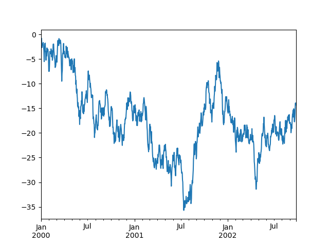
In [128]: ts = pd.Series(np.random.randn(1000), index=pd.date_range("1/1/2000", periods=1000))

In [129]: ts = ts.cumsum()

In [130]: ts.plot();
Note
When using Jupyter, the plot will appear using plot(). Otherwise use
matplotlib.pyplot.show to show it or
matplotlib.pyplot.savefig to write it to a file.
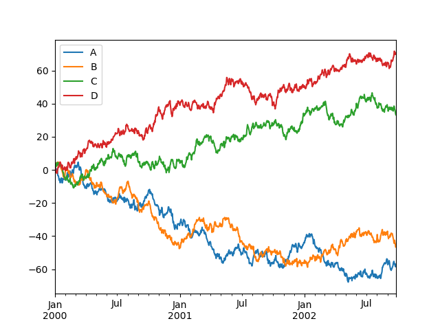
plot() plots all columns:
In [131]: df = pd.DataFrame(
   .....:     np.random.randn(1000, 4), index=ts.index, columns=["A", "B", "C", "D"]
   .....: )
   .....:

In [132]: df = df.cumsum()

In [133]: plt.figure();

In [134]: df.plot();

In [135]: plt.legend(loc='best');
Importing and exporting data#
See the IO Tools section.
CSV#
Writing to a csv file: using DataFrame.to_csv()
In [136]: df = pd.DataFrame(np.random.randint(0, 5, (10, 5)))

In [137]: df.to_csv("foo.csv")
Reading from a csv file: using read_csv()
In [138]: pd.read_csv("foo.csv")
Out[138]:
   Unnamed: 0  0  1  2  3  4
0           0  4  3  1  1  2
1           1  1  0  2  3  2
2           2  1  4  2  1  2
3           3  0  4  0  2  2
4           4  4  2  2  3  4
5           5  4  0  4  3  1
6           6  2  1  2  0  3
7           7  4  0  4  4  4
8           8  4  4  1  0  1
9           9  0  4  3  0  3
Parquet#
Writing to a Parquet file:
In [139]: df.to_parquet("foo.parquet")
Reading from a Parquet file Store using read_parquet():
In [140]: pd.read_parquet("foo.parquet")
Out[140]:
   0  1  2  3  4
0  4  3  1  1  2
1  1  0  2  3  2
2  1  4  2  1  2
3  0  4  0  2  2
4  4  2  2  3  4
5  4  0  4  3  1
6  2  1  2  0  3
7  4  0  4  4  4
8  4  4  1  0  1
9  0  4  3  0  3
Excel#
Reading and writing to Excel.
Writing to an excel file using DataFrame.to_excel():
In [141]: df.to_excel("foo.xlsx", sheet_name="Sheet1")
Reading from an excel file using read_excel():
In [142]: pd.read_excel("foo.xlsx", "Sheet1", index_col=None, na_values=["NA"])
Out[142]:
   Unnamed: 0  0  1  2  3  4
0           0  4  3  1  1  2
1           1  1  0  2  3  2
2           2  1  4  2  1  2
3           3  0  4  0  2  2
4           4  4  2  2  3  4
5           5  4  0  4  3  1
6           6  2  1  2  0  3
7           7  4  0  4  4  4
8           8  4  4  1  0  1
9           9  0  4  3  0  3
Gotchas#
If you are attempting to perform a boolean operation on a Series or DataFrame
you might see an exception like:
In [143]: if pd.Series([False, True, False]):
   .....:      print("I was true")
   .....:
---------------------------------------------------------------------------
ValueError                                Traceback (most recent call last)
Cell In[143], line 1
----> 1 if pd.Series([False, True, False]):
      2      print("I was true")

File ~/work/pandas/pandas/pandas/core/generic.py:1501, in NDFrame.__bool__(self)
   1499     @final
   1500     def __bool__(self) -> NoReturn:
-> 1501         raise ValueError(
   1502             f"The truth value of a {type(self).__name__} is ambiguous. "
   1503             "Use a.empty, a.bool(), a.item(), a.any() or a.all()."
   1504         )

ValueError: The truth value of a Series is ambiguous. Use a.empty, a.bool(), a.item(), a.any() or a.all().
See Comparisons and Gotchas for an explanation and what to do.