Group By: split-apply-combine
By “group by” we are referring to a process involving one or more of the following steps
- Splitting the data into groups based on some criteria
- Applying a function to each group independently
- Combining the results into a data structure
Of these, the split step is the most straightforward. In fact, in many situations you may wish to split the data set into groups and do something with those groups yourself. In the apply step, we might wish to one of the following:
Aggregation: computing a summary statistic (or statistics) about each group. Some examples:
- Compute group sums or means
- Compute group sizes / counts
Transformation: perform some group-specific computations and return a like-indexed. Some examples:
- Standardizing data (zscore) within group
- Filling NAs within groups with a value derived from each group
Filtration: discard some groups, according to a group-wise computation that evaluates True or False. Some examples:
- Discarding data that belongs to groups with only a few members
- Filtering out data based on the group sum or mean
Some combination of the above: GroupBy will examine the results of the apply step and try to return a sensibly combined result if it doesn’t fit into either of the above two categories
Since the set of object instance method on pandas data structures are generally rich and expressive, we often simply want to invoke, say, a DataFrame function on each group. The name GroupBy should be quite familiar to those who have used a SQL-based tool (or itertools), in which you can write code like:
SELECT Column1, Column2, mean(Column3), sum(Column4)
FROM SomeTable
GROUP BY Column1, Column2
We aim to make operations like this natural and easy to express using pandas. We’ll address each area of GroupBy functionality then provide some non-trivial examples / use cases.
See the cookbook for some advanced strategies
Splitting an object into groups
pandas objects can be split on any of their axes. The abstract definition of grouping is to provide a mapping of labels to group names. To create a GroupBy object (more on what the GroupBy object is later), you do the following:
>>> grouped = obj.groupby(key)
>>> grouped = obj.groupby(key, axis=1)
>>> grouped = obj.groupby([key1, key2])
The mapping can be specified many different ways:
- A Python function, to be called on each of the axis labels
- A list or NumPy array of the same length as the selected axis
- A dict or Series, providing a label -> group name mapping
- For DataFrame objects, a string indicating a column to be used to group. Of course df.groupby('A') is just syntactic sugar for df.groupby(df['A']), but it makes life simpler
- A list of any of the above things
Collectively we refer to the grouping objects as the keys. For example, consider the following DataFrame:
In [1]: df = DataFrame({'A' : ['foo', 'bar', 'foo', 'bar',
   ...:                        'foo', 'bar', 'foo', 'foo'],
   ...:                 'B' : ['one', 'one', 'two', 'three',
   ...:                        'two', 'two', 'one', 'three'],
   ...:                 'C' : randn(8), 'D' : randn(8)})
   ...:

In [2]: df

     A      B         C         D
0  foo    one  0.469112 -0.861849
1  bar    one -0.282863 -2.104569
2  foo    two -1.509059 -0.494929
3  bar  three -1.135632  1.071804
4  foo    two  1.212112  0.721555
5  bar    two -0.173215 -0.706771
6  foo    one  0.119209 -1.039575
7  foo  three -1.044236  0.271860
[8 rows x 4 columns]
We could naturally group by either the A or B columns or both:
In [3]: grouped = df.groupby('A')

In [4]: grouped = df.groupby(['A', 'B'])
These will split the DataFrame on its index (rows). We could also split by the columns:
In [5]: def get_letter_type(letter):
   ...:     if letter.lower() in 'aeiou':
   ...:         return 'vowel'
   ...:     else:
   ...:         return 'consonant'
   ...:

In [6]: grouped = df.groupby(get_letter_type, axis=1)
Starting with 0.8, pandas Index objects now supports duplicate values. If a non-unique index is used as the group key in a groupby operation, all values for the same index value will be considered to be in one group and thus the output of aggregation functions will only contain unique index values:
In [7]: lst = [1, 2, 3, 1, 2, 3]

In [8]: s = Series([1, 2, 3, 10, 20, 30], lst)

In [9]: grouped = s.groupby(level=0)

In [10]: grouped.first()

1    1
2    2
3    3
dtype: int64

In [11]: grouped.last()

1    10
2    20
3    30
dtype: int64

In [12]: grouped.sum()

1    11
2    22
3    33
dtype: int64
Note that no splitting occurs until it’s needed. Creating the GroupBy object only verifies that you’ve passed a valid mapping.
Note
Many kinds of complicated data manipulations can be expressed in terms of GroupBy operations (though can’t be guaranteed to be the most efficient). You can get quite creative with the label mapping functions.
GroupBy object attributes
The groups attribute is a dict whose keys are the computed unique groups and corresponding values being the axis labels belonging to each group. In the above example we have:
In [13]: df.groupby('A').groups
{'bar': [1, 3, 5], 'foo': [0, 2, 4, 6, 7]}

In [14]: df.groupby(get_letter_type, axis=1).groups
{'consonant': ['B', 'C', 'D'], 'vowel': ['A']}
Calling the standard Python len function on the GroupBy object just returns the length of the groups dict, so it is largely just a convenience:
In [15]: grouped = df.groupby(['A', 'B'])

In [16]: grouped.groups

{('bar', 'one'): [1],
 ('bar', 'three'): [3],
 ('bar', 'two'): [5],
 ('foo', 'one'): [0, 6],
 ('foo', 'three'): [7],
 ('foo', 'two'): [2, 4]}

In [17]: len(grouped)
6
By default the group keys are sorted during the groupby operation. You may however pass sort=False for potential speedups:
In [18]: df2 = DataFrame({'X' : ['B', 'B', 'A', 'A'], 'Y' : [1, 2, 3, 4]})

In [19]: df2.groupby(['X'], sort=True).sum()

   Y
X
A  7
B  3
[2 rows x 1 columns]

In [20]: df2.groupby(['X'], sort=False).sum()

   Y
X
B  3
A  7
[2 rows x 1 columns]
GroupBy will tab complete column names (and other attributes)
In [21]: df

            gender     height      weight
2000-01-01    male  42.849980  157.500553
2000-01-02    male  49.607315  177.340407
2000-01-03    male  56.293531  171.524640
2000-01-04  female  48.421077  144.251986
2000-01-05    male  46.556882  152.526206
2000-01-06  female  68.448851  168.272968
2000-01-07    male  70.757698  136.431469
2000-01-08  female  58.909500  176.499753
2000-01-09  female  76.435631  174.094104
2000-01-10    male  45.306120  177.540920
[10 rows x 3 columns]

In [22]: gb = df.groupby('gender')
In [23]: gb.<TAB>
gb.agg        gb.boxplot    gb.cummin     gb.describe   gb.filter     gb.get_group  gb.height     gb.last       gb.median     gb.ngroups    gb.plot       gb.rank       gb.std        gb.transform
gb.aggregate  gb.count      gb.cumprod    gb.dtype      gb.first      gb.groups     gb.hist       gb.max        gb.min        gb.nth        gb.prod       gb.resample   gb.sum        gb.var
gb.apply      gb.cummax     gb.cumsum     gb.fillna     gb.gender     gb.head       gb.indices    gb.mean       gb.name       gb.ohlc       gb.quantile   gb.size       gb.tail       gb.weight
GroupBy with MultiIndex
With hierarchically-indexed data, it’s quite natural to group by one of the levels of the hierarchy.
In [24]: s

first  second
bar    one      -0.575247
       two       0.254161
baz    one      -1.143704
       two       0.215897
foo    one       1.193555
       two      -0.077118
qux    one      -0.408530
       two      -0.862495
dtype: float64

In [25]: grouped = s.groupby(level=0)

In [26]: grouped.sum()

first
bar     -0.321085
baz     -0.927807
foo      1.116437
qux     -1.271025
dtype: float64
If the MultiIndex has names specified, these can be passed instead of the level number:
In [27]: s.groupby(level='second').sum()

second
one      -0.933926
two      -0.469555
dtype: float64
The aggregation functions such as sum will take the level parameter directly. Additionally, the resulting index will be named according to the chosen level:
In [28]: s.sum(level='second')

second
one      -0.933926
two      -0.469555
dtype: float64
Also as of v0.6, grouping with multiple levels is supported.
In [29]: s

first  second  third
bar    doo     one      1.346061
               two      1.511763
baz    bee     one      1.627081
               two     -0.990582
foo    bop     one     -0.441652
               two      1.211526
qux    bop     one      0.268520
               two      0.024580
dtype: float64

In [30]: s.groupby(level=['first','second']).sum()

first  second
bar    doo       2.857824
baz    bee       0.636499
foo    bop       0.769873
qux    bop       0.293100
dtype: float64
More on the sum function and aggregation later.
DataFrame column selection in GroupBy
Once you have created the GroupBy object from a DataFrame, for example, you might want to do something different for each of the columns. Thus, using [] similar to getting a column from a DataFrame, you can do:
In [31]: grouped = df.groupby(['A'])

In [32]: grouped_C = grouped['C']

In [33]: grouped_D = grouped['D']
This is mainly syntactic sugar for the alternative and much more verbose:
In [34]: df['C'].groupby(df['A'])
<pandas.core.groupby.SeriesGroupBy object at 0xf27b410>
Additionally this method avoids recomputing the internal grouping information derived from the passed key.
Iterating through groups
With the GroupBy object in hand, iterating through the grouped data is very natural and functions similarly to itertools.groupby:
In [35]: grouped = df.groupby('A')

In [36]: for name, group in grouped:
   ....:        print(name)
   ....:        print(group)
   ....:
bar
     A      B         C         D
1  bar    one -0.042379 -0.089329
3  bar  three -0.009920 -0.945867
5  bar    two  0.495767  1.956030
[3 rows x 4 columns]
foo
     A      B         C         D
0  foo    one -0.919854 -1.131345
2  foo    two  1.247642  0.337863
4  foo    two  0.290213 -0.932132
6  foo    one  0.362949  0.017587
7  foo  three  1.548106 -0.016692
[5 rows x 4 columns]
In the case of grouping by multiple keys, the group name will be a tuple:
In [37]: for name, group in df.groupby(['A', 'B']):
   ....:        print(name)
   ....:        print(group)
   ....:
('bar', 'one')
     A    B         C         D
1  bar  one -0.042379 -0.089329
[1 rows x 4 columns]
('bar', 'three')
     A      B        C         D
3  bar  three -0.00992 -0.945867
[1 rows x 4 columns]
('bar', 'two')
     A    B         C        D
5  bar  two  0.495767  1.95603
[1 rows x 4 columns]
('foo', 'one')
     A    B         C         D
0  foo  one -0.919854 -1.131345
6  foo  one  0.362949  0.017587
[2 rows x 4 columns]
('foo', 'three')
     A      B         C         D
7  foo  three  1.548106 -0.016692
[1 rows x 4 columns]
('foo', 'two')
     A    B         C         D
2  foo  two  1.247642  0.337863
4  foo  two  0.290213 -0.932132
[2 rows x 4 columns]
It’s standard Python-fu but remember you can unpack the tuple in the for loop statement if you wish: for (k1, k2), group in grouped:.
Aggregation
Once the GroupBy object has been created, several methods are available to perform a computation on the grouped data. An obvious one is aggregation via the aggregate or equivalently agg method:
In [38]: grouped = df.groupby('A')

In [39]: grouped.aggregate(np.sum)

            C         D
A
bar  0.443469  0.920834
foo  2.529056 -1.724719
[2 rows x 2 columns]

In [40]: grouped = df.groupby(['A', 'B'])

In [41]: grouped.aggregate(np.sum)

                  C         D
A   B
bar one   -0.042379 -0.089329
    three -0.009920 -0.945867
    two    0.495767  1.956030
foo one   -0.556905 -1.113758
    three  1.548106 -0.016692
    two    1.537855 -0.594269
[6 rows x 2 columns]
As you can see, the result of the aggregation will have the group names as the new index along the grouped axis. In the case of multiple keys, the result is a MultiIndex by default, though this can be changed by using the as_index option:
In [42]: grouped = df.groupby(['A', 'B'], as_index=False)

In [43]: grouped.aggregate(np.sum)

     A      B         C         D
0  bar    one -0.042379 -0.089329
1  bar  three -0.009920 -0.945867
2  bar    two  0.495767  1.956030
3  foo    one -0.556905 -1.113758
4  foo  three  1.548106 -0.016692
5  foo    two  1.537855 -0.594269
[6 rows x 4 columns]

In [44]: df.groupby('A', as_index=False).sum()

     A         C         D
0  bar  0.443469  0.920834
1  foo  2.529056 -1.724719
[2 rows x 3 columns]
Note that you could use the reset_index DataFrame function to achieve the same result as the column names are stored in the resulting MultiIndex:
In [45]: df.groupby(['A', 'B']).sum().reset_index()

     A      B         C         D
0  bar    one -0.042379 -0.089329
1  bar  three -0.009920 -0.945867
2  bar    two  0.495767  1.956030
3  foo    one -0.556905 -1.113758
4  foo  three  1.548106 -0.016692
5  foo    two  1.537855 -0.594269
[6 rows x 4 columns]
Another simple aggregation example is to compute the size of each group. This is included in GroupBy as the size method. It returns a Series whose index are the group names and whose values are the sizes of each group.
In [46]: grouped.size()

A    B
bar  one      1
     three    1
     two      1
foo  one      2
     three    1
     two      2
dtype: int64
Applying multiple functions at once
With grouped Series you can also pass a list or dict of functions to do aggregation with, outputting a DataFrame:
In [47]: grouped = df.groupby('A')

In [48]: grouped['C'].agg([np.sum, np.mean, np.std])

          sum      mean       std
A
bar  0.443469  0.147823  0.301765
foo  2.529056  0.505811  0.966450
[2 rows x 3 columns]
If a dict is passed, the keys will be used to name the columns. Otherwise the function’s name (stored in the function object) will be used.
In [49]: grouped['D'].agg({'result1' : np.sum,
   ....:                   'result2' : np.mean})
   ....:

      result2   result1
A
bar  0.306945  0.920834
foo -0.344944 -1.724719
[2 rows x 2 columns]
On a grouped DataFrame, you can pass a list of functions to apply to each column, which produces an aggregated result with a hierarchical index:
In [50]: grouped.agg([np.sum, np.mean, np.std])

            C                             D
          sum      mean       std       sum      mean       std
A
bar  0.443469  0.147823  0.301765  0.920834  0.306945  1.490982
foo  2.529056  0.505811  0.966450 -1.724719 -0.344944  0.645875
[2 rows x 6 columns]
Passing a dict of functions has different behavior by default, see the next section.
Applying different functions to DataFrame columns
By passing a dict to aggregate you can apply a different aggregation to the columns of a DataFrame:
In [51]: grouped.agg({'C' : np.sum,
   ....:              'D' : lambda x: np.std(x, ddof=1)})
   ....:

            C         D
A
bar  0.443469  1.490982
foo  2.529056  0.645875
[2 rows x 2 columns]
The function names can also be strings. In order for a string to be valid it must be either implemented on GroupBy or available via dispatching:
In [52]: grouped.agg({'C' : 'sum', 'D' : 'std'})

            C         D
A
bar  0.443469  1.490982
foo  2.529056  0.645875
[2 rows x 2 columns]
Cython-optimized aggregation functions
Some common aggregations, currently only sum, mean, and std, have optimized Cython implementations:
In [53]: df.groupby('A').sum()

            C         D
A
bar  0.443469  0.920834
foo  2.529056 -1.724719
[2 rows x 2 columns]

In [54]: df.groupby(['A', 'B']).mean()

                  C         D
A   B
bar one   -0.042379 -0.089329
    three -0.009920 -0.945867
    two    0.495767  1.956030
foo one   -0.278452 -0.556879
    three  1.548106 -0.016692
    two    0.768928 -0.297134
[6 rows x 2 columns]
Of course sum and mean are implemented on pandas objects, so the above code would work even without the special versions via dispatching (see below).
Transformation
The transform method returns an object that is indexed the same (same size) as the one being grouped. Thus, the passed transform function should return a result that is the same size as the group chunk. For example, suppose we wished to standardize the data within each group:
In [55]: index = date_range('10/1/1999', periods=1100)

In [56]: ts = Series(np.random.normal(0.5, 2, 1100), index)

In [57]: ts = rolling_mean(ts, 100, 100).dropna()

In [58]: ts.head()

2000-01-08    0.779333
2000-01-09    0.778852
2000-01-10    0.786476
2000-01-11    0.782797
2000-01-12    0.798110
Freq: D, dtype: float64

In [59]: ts.tail()

2002-09-30    0.660294
2002-10-01    0.631095
2002-10-02    0.673601
2002-10-03    0.709213
2002-10-04    0.719369
Freq: D, dtype: float64

In [60]: key = lambda x: x.year

In [61]: zscore = lambda x: (x - x.mean()) / x.std()

In [62]: transformed = ts.groupby(key).transform(zscore)
We would expect the result to now have mean 0 and standard deviation 1 within each group, which we can easily check:
# Original Data
In [63]: grouped = ts.groupby(key)

In [64]: grouped.mean()

2000    0.442441
2001    0.526246
2002    0.459365
dtype: float64

In [65]: grouped.std()

2000    0.131752
2001    0.210945
2002    0.128753
dtype: float64

# Transformed Data
In [66]: grouped_trans = transformed.groupby(key)

In [67]: grouped_trans.mean()

2000    1.168208e-15
2001    1.454544e-15
2002    1.726657e-15
dtype: float64

In [68]: grouped_trans.std()

2000    1
2001    1
2002    1
dtype: float64
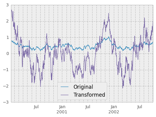
We can also visually compare the original and transformed data sets.
In [69]: compare = DataFrame({'Original': ts, 'Transformed': transformed})

In [70]: compare.plot()
<matplotlib.axes.AxesSubplot at 0xfecf450>
Another common data transform is to replace missing data with the group mean.
In [71]: data_df

           A         B         C
0   1.539708 -1.166480  0.533026
1   1.302092 -0.505754       NaN
2  -0.371983  1.104803 -0.651520
3  -1.309622  1.118697 -1.161657
4  -1.924296  0.396437  0.812436
5   0.815643  0.367816 -0.469478
6  -0.030651  1.376106 -0.645129
7   0.798630 -1.729858  0.392067
8  -0.347401 -0.429063  1.792958
9  -0.431059  1.605289 -3.302946
10  0.434332 -1.302198  0.756527
11 -0.349926       NaN  0.304228
12       NaN -0.024779       NaN
13  1.026076 -0.151723 -1.136601
14  0.611215 -0.897508  0.022300
         ...       ...       ...
[1000 rows x 3 columns]

In [72]: countries = np.array(['US', 'UK', 'GR', 'JP'])

In [73]: key = countries[np.random.randint(0, 4, 1000)]

In [74]: grouped = data_df.groupby(key)

# Non-NA count in each group
In [75]: grouped.count()

      A    B    C
GR  209  217  189
JP  240  255  217
UK  216  231  193
US  239  250  217
[4 rows x 3 columns]

In [76]: f = lambda x: x.fillna(x.mean())

In [77]: transformed = grouped.transform(f)
We can verify that the group means have not changed in the transformed data and that the transformed data contains no NAs.
In [78]: grouped_trans = transformed.groupby(key)

In [79]: grouped.mean() # original group means

           A         B         C
GR -0.098371 -0.015420  0.068053
JP  0.069025  0.023100 -0.077324
UK  0.034069 -0.052580 -0.116525
US  0.058664 -0.020399  0.028603
[4 rows x 3 columns]

In [80]: grouped_trans.mean() # transformation did not change group means

           A         B         C
GR -0.098371 -0.015420  0.068053
JP  0.069025  0.023100 -0.077324
UK  0.034069 -0.052580 -0.116525
US  0.058664 -0.020399  0.028603
[4 rows x 3 columns]

In [81]: grouped.count() # original has some missing data points

      A    B    C
GR  209  217  189
JP  240  255  217
UK  216  231  193
US  239  250  217
[4 rows x 3 columns]

In [82]: grouped_trans.count() # counts after transformation

      A    B    C
GR  228  228  228
JP  267  267  267
UK  247  247  247
US  258  258  258
[4 rows x 3 columns]

In [83]: grouped_trans.size() # Verify non-NA count equals group size

GR    228
JP    267
UK    247
US    258
dtype: int64
Filtration
New in version 0.12.
The filter method returns a subset of the original object. Suppose we want to take only elements that belong to groups with a group sum greater than 2.
In [84]: sf = Series([1, 1, 2, 3, 3, 3])

In [85]: sf.groupby(sf).filter(lambda x: x.sum() > 2)

3    3
4    3
5    3
dtype: int64
The argument of filter must be a function that, applied to the group as a whole, returns True or False.
Another useful operation is filtering out elements that belong to groups with only a couple members.
In [86]: dff = DataFrame({'A': np.arange(8), 'B': list('aabbbbcc')})

In [87]: dff.groupby('B').filter(lambda x: len(x) > 2)

   A  B
2  2  b
3  3  b
4  4  b
5  5  b
[4 rows x 2 columns]
Alternatively, instead of dropping the offending groups, we can return a like-indexed objects where the groups that do not pass the filter are filled with NaNs.
In [88]: dff.groupby('B').filter(lambda x: len(x) > 2, dropna=False)

    A    B
0 NaN  NaN
1 NaN  NaN
2   2    b
3   3    b
4   4    b
5   5    b
6 NaN  NaN
7 NaN  NaN
[8 rows x 2 columns]
For dataframes with multiple columns, filters should explicitly specify a column as the filter criterion.
In [89]: dff['C'] = np.arange(8)

In [90]: dff.groupby('B').filter(lambda x: len(x['C']) > 2)

   A  B  C
2  2  b  2
3  3  b  3
4  4  b  4
5  5  b  5
[4 rows x 3 columns]
Dispatching to instance methods
When doing an aggregation or transformation, you might just want to call an instance method on each data group. This is pretty easy to do by passing lambda functions:
In [91]: grouped = df.groupby('A')

In [92]: grouped.agg(lambda x: x.std())

      B         C         D
A
bar NaN  0.301765  1.490982
foo NaN  0.966450  0.645875
[2 rows x 3 columns]
But, it’s rather verbose and can be untidy if you need to pass additional arguments. Using a bit of metaprogramming cleverness, GroupBy now has the ability to “dispatch” method calls to the groups:
In [93]: grouped.std()

            C         D
A
bar  0.301765  1.490982
foo  0.966450  0.645875
[2 rows x 2 columns]
What is actually happening here is that a function wrapper is being generated. When invoked, it takes any passed arguments and invokes the function with any arguments on each group (in the above example, the std function). The results are then combined together much in the style of agg and transform (it actually uses apply to infer the gluing, documented next). This enables some operations to be carried out rather succinctly:
In [94]: tsdf = DataFrame(randn(1000, 3),
   ....:                  index=date_range('1/1/2000', periods=1000),
   ....:                  columns=['A', 'B', 'C'])
   ....:

In [95]: tsdf.ix[::2] = np.nan

In [96]: grouped = tsdf.groupby(lambda x: x.year)

In [97]: grouped.fillna(method='pad')

                   A         B         C
2000-01-01       NaN       NaN       NaN
2000-01-02 -0.353501 -0.080957 -0.876864
2000-01-03 -0.353501 -0.080957 -0.876864
2000-01-04  0.050976  0.044273 -0.559849
2000-01-05  0.050976  0.044273 -0.559849
2000-01-06  0.030091  0.186460 -0.680149
2000-01-07  0.030091  0.186460 -0.680149
2000-01-08 -0.882655  0.661310  1.317217
2000-01-09 -0.882655  0.661310  1.317217
2000-01-10  0.008021  0.572938  0.309048
2000-01-11  0.008021  0.572938  0.309048
2000-01-12 -0.818637 -2.130013 -1.346086
2000-01-13 -0.818637 -2.130013 -1.346086
2000-01-14  0.315112 -1.667438 -0.363184
2000-01-15  0.315112 -1.667438 -0.363184
                 ...       ...       ...
[1000 rows x 3 columns]
In this example, we chopped the collection of time series into yearly chunks then independently called fillna on the groups.
Flexible apply
Some operations on the grouped data might not fit into either the aggregate or transform categories. Or, you may simply want GroupBy to infer how to combine the results. For these, use the apply function, which can be substituted for both aggregate and transform in many standard use cases. However, apply can handle some exceptional use cases, for example:
In [98]: df

     A      B         C         D
0  foo    one -0.919854 -1.131345
1  bar    one -0.042379 -0.089329
2  foo    two  1.247642  0.337863
3  bar  three -0.009920 -0.945867
4  foo    two  0.290213 -0.932132
5  bar    two  0.495767  1.956030
6  foo    one  0.362949  0.017587
7  foo  three  1.548106 -0.016692
[8 rows x 4 columns]

In [99]: grouped = df.groupby('A')

# could also just call .describe()
In [100]: grouped['C'].apply(lambda x: x.describe())

A
bar  count    3.000000
     mean     0.147823
     std      0.301765
     min     -0.042379
     25%     -0.026149
...
foo  std    0.966450
     min   -0.919854
     25%    0.290213
     50%    0.362949
     75%    1.247642
     max    1.548106
Length: 16, dtype: float64
The dimension of the returned result can also change:
In [101]: grouped = df.groupby('A')['C']

In [102]: def f(group):
   .....:     return DataFrame({'original' : group,
   .....:                       'demeaned' : group - group.mean()})
   .....:

In [103]: grouped.apply(f)

   demeaned  original
0 -1.425665 -0.919854
1 -0.190202 -0.042379
2  0.741831  1.247642
3 -0.157743 -0.009920
4 -0.215598  0.290213
5  0.347944  0.495767
6 -0.142862  0.362949
7  1.042295  1.548106
[8 rows x 2 columns]
apply on a Series can operate on a returned value from the applied function, that is itself a series, and possibly upcast the result to a DataFrame
In [104]: def f(x):
   .....:   return Series([ x, x**2 ], index = ['x', 'x^s'])
   .....:

In [105]: s = Series(np.random.rand(5))

In [106]: s

0    0.321438
1    0.493496
2    0.139505
3    0.910103
4    0.194158
dtype: float64

In [107]: s.apply(f)

          x       x^s
0  0.321438  0.103323
1  0.493496  0.243538
2  0.139505  0.019462
3  0.910103  0.828287
4  0.194158  0.037697
[5 rows x 2 columns]
Other useful features
Automatic exclusion of “nuisance” columns
Again consider the example DataFrame we’ve been looking at:
In [108]: df

     A      B         C         D
0  foo    one -0.919854 -1.131345
1  bar    one -0.042379 -0.089329
2  foo    two  1.247642  0.337863
3  bar  three -0.009920 -0.945867
4  foo    two  0.290213 -0.932132
5  bar    two  0.495767  1.956030
6  foo    one  0.362949  0.017587
7  foo  three  1.548106 -0.016692
[8 rows x 4 columns]
Supposed we wished to compute the standard deviation grouped by the A column. There is a slight problem, namely that we don’t care about the data in column B. We refer to this as a “nuisance” column. If the passed aggregation function can’t be applied to some columns, the troublesome columns will be (silently) dropped. Thus, this does not pose any problems:
In [109]: df.groupby('A').std()

            C         D
A
bar  0.301765  1.490982
foo  0.966450  0.645875
[2 rows x 2 columns]
NA group handling
If there are any NaN values in the grouping key, these will be automatically excluded. So there will never be an “NA group”. This was not the case in older versions of pandas, but users were generally discarding the NA group anyway (and supporting it was an implementation headache).
Grouping with ordered factors
Categorical variables represented as instance of pandas’s Categorical class can be used as group keys. If so, the order of the levels will be preserved:
In [110]: data = Series(np.random.randn(100))

In [111]: factor = qcut(data, [0, .25, .5, .75, 1.])

In [112]: data.groupby(factor).mean()

[-2.644, -0.523]   -1.362896
(-0.523, 0.0296]   -0.260266
(0.0296, 0.654]     0.361802
(0.654, 2.21]       1.073801
dtype: float64
Enumerate group items
New in version 0.13.0.
To see the order in which each row appears within its group, use the cumcount method:
In [113]: df = pd.DataFrame(list('aaabba'), columns=['A'])

In [114]: df

   A
0  a
1  a
2  a
3  b
4  b
5  a
[6 rows x 1 columns]

In [115]: df.groupby('A').cumcount()

0    0
1    1
2    2
3    0
4    1
5    3
dtype: int64

In [116]: df.groupby('A').cumcount(ascending=False)  # kwarg only

0    3
1    2
2    1
3    1
4    0
5    0
dtype: int64