pandas.Series.plot.kde

Series.plot.kde(bw_method=None, ind=None, weights=None, **kwargs)

Generate Kernel Density Estimate plot using Gaussian kernels.

In statistics, kernel density estimation (KDE) is a non-parametric way to estimate the probability density function (PDF) of a random variable. This function uses Gaussian kernels and includes automatic bandwidth determination.

Parameters:

bw_methodstr, scalar or callable, optional

The method used to calculate the estimator bandwidth. This can be ‘scott’, ‘silverman’, a scalar constant or a callable. If None (default), ‘scott’ is used. See scipy.stats.gaussian_kde for more information.

indNumPy array or int, optional

Evaluation points for the estimated PDF. If None (default), 1000 equally spaced points are used. If ind is a NumPy array, the KDE is evaluated at the points passed. If ind is an integer, ind number of equally spaced points are used.

weightsNumPy array, optional

Weights of datapoints. This must be the same shape as datapoints. If None (default), the samples are assumed to be equally weighted.

**kwargs

Additional keyword arguments are documented in DataFrame.plot().

Returns:

matplotlib.axes.Axes or numpy.ndarray of them

The matplotlib axes containing the KDE plot.

See also

scipy.stats.gaussian_kde

Representation of a kernel-density estimate using Gaussian kernels. This is the function used internally to estimate the PDF.

Examples

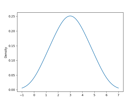
Given a Series of points randomly sampled from an unknown distribution, estimate its PDF using KDE with automatic bandwidth determination and plot the results, evaluating them at 1000 equally spaced points (default):

>>> s = pd.Series([1, 2, 2.5, 3, 3.5, 4, 5])
>>> ax = s.plot.kde()

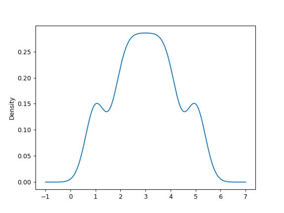
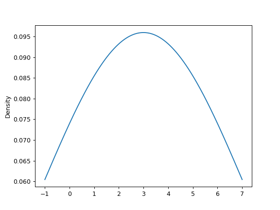
A scalar bandwidth can be specified. Using a small bandwidth value can lead to over-fitting, while using a large bandwidth value may result in under-fitting:

>>> ax = s.plot.kde(bw_method=0.3)

>>> ax = s.plot.kde(bw_method=3)

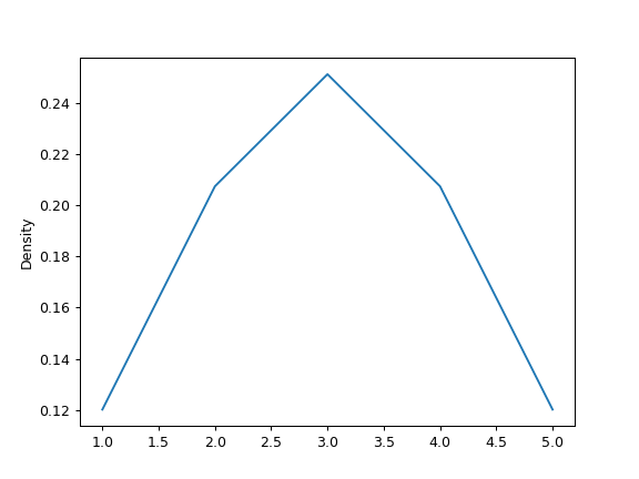
Finally, the ind parameter determines the evaluation points for the plot of the estimated PDF:

>>> ax = s.plot.kde(ind=[1, 2, 3, 4, 5])

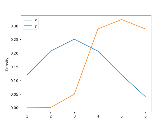
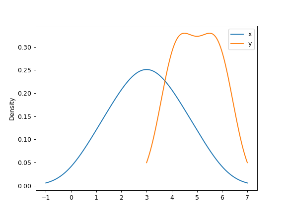
For DataFrame, it works in the same way:

>>> df = pd.DataFrame(
...     {
...         "x": [1, 2, 2.5, 3, 3.5, 4, 5],
...         "y": [4, 4, 4.5, 5, 5.5, 6, 6],
...     }
... )
>>> ax = df.plot.kde()

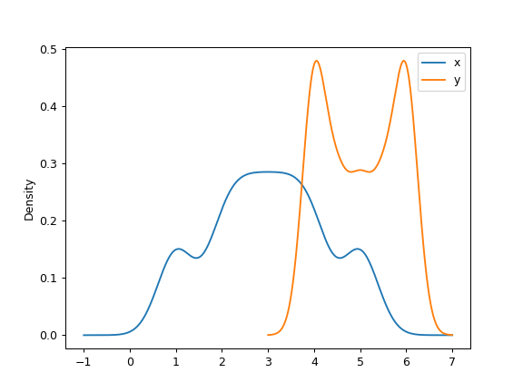
A scalar bandwidth can be specified. Using a small bandwidth value can lead to over-fitting, while using a large bandwidth value may result in under-fitting:

>>> ax = df.plot.kde(bw_method=0.3)

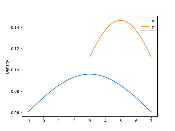
>>> ax = df.plot.kde(bw_method=3)

Finally, the ind parameter determines the evaluation points for the plot of the estimated PDF:

>>> ax = df.plot.kde(ind=[1, 2, 3, 4, 5, 6])